如何使用SQL Server Reporting Services将数据格式转换为有价值的数据集

最新推荐文章于 2023-06-11 21:28:03 发布

culuo4781

最新推荐文章于 2023-06-11 21:28:03 发布

阅读量519

点赞数

文章标签： java sqlserver sql python 脚本语言

原文链接：https://www.sqlshack.com/convert-data-format-into-valuable-dataset-using-sql-server-reporting-services/

版权

介绍 ( Introduction )

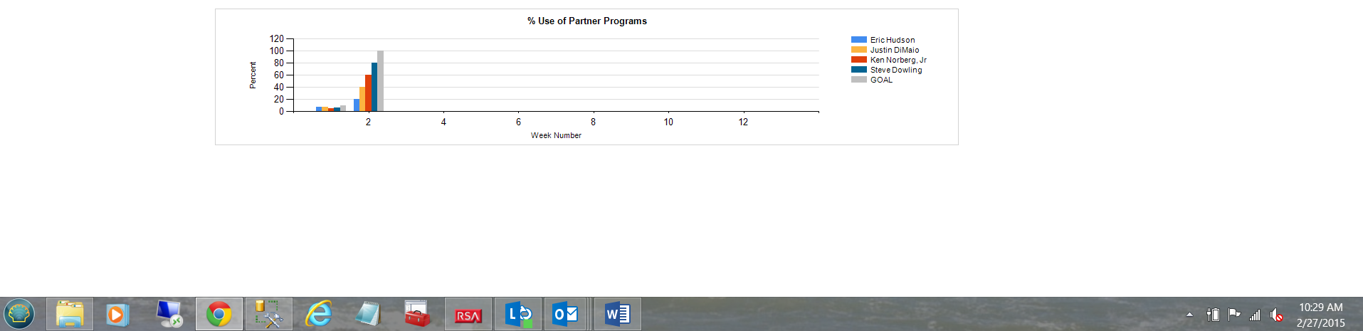
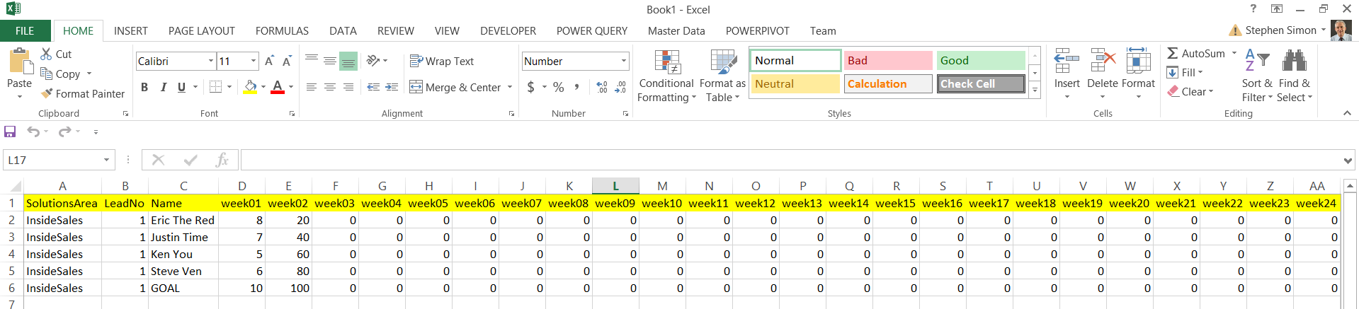
Oft times we are forced into situations where we must clearly think outside of the box. In today’s “get together”, we are going to discuss a challenge that I encountered during the last week of February of this year. The client had been charting weekly business calls placed by his sales reps. Our client had been tracking these results within an Excel spreadsheet (see the screen dump below) and he would be using this spreadsheet to report the sales reps progress going forward. My task was to source this data for the corporate reports in Reporting Services, from this spreadsheet and do so on a weekly basis. The client, being resistant to change, was not willing to change the format of the spreadsheet to something more conducive to be utilized by the chart that he wished to produce (see immediately below).

很多时候，我们被迫陷入必须明确思考的情况。在今天的“聚在一起”中，我们将讨论我在今年2月的最后一周遇到的挑战。该客户一直在绘制由其销售代表发出的每周商务电话。我们的客户一直在Excel电子表格中跟踪这些结果（请参见下面的屏幕转储），他将使用该电子表格报告销售代表的进度。我的任务是每周从此电子表格中为Reporting Services中的公司报告提供此数据。拒绝更改的客户不愿意将电子表格的格式更改为更有利于他希望生成的图表使用的格式（请参见下文）。

Another challenge was the efficient and effective usage of the report real estate. After having produced the POC, we soon realized that a full plot of 52 weeks would not be a viable option due to the vast amount of data and employees to be represented in such a small area. At the end of the day, we opted to show the current quarter’s data based upon logic placed within the query code which would determine the current quarter, calculated at runtime.

另一个挑战是如何有效利用报表资源。制作了POC之后，我们很快意识到，由于要在如此小的区域内代表大量数据和员工，所以要花52周的完整时间是不可行的选择。在一天结束时，我们选择基于放置在查询代码中的逻辑来显示当前季度的数据，该逻辑将确定在运行时计算的当前季度。

A sample of the finished chart may be seen above, whilst the format of the raw data from the user’s spreadsheet may be seen below:

可以从上方看到完成图表的示例，而从用户电子表格获得的原始数据的格式可以从下面看到：

All said and done, the data had to be pivoted and this is our challenge for today’s chat.

总而言之，数据必须进行数据透视，这是我们今天聊天的挑战。

入门 ( Getting started )

创建从用户电子表格到暂存表的负载 ( Creating our load from the users spreadsheet to the staging table )

Opening SQL Server Data Tools we create a new Integration Services project.

打开SQL Server数据工具，我们创建一个新的Integration Services项目。

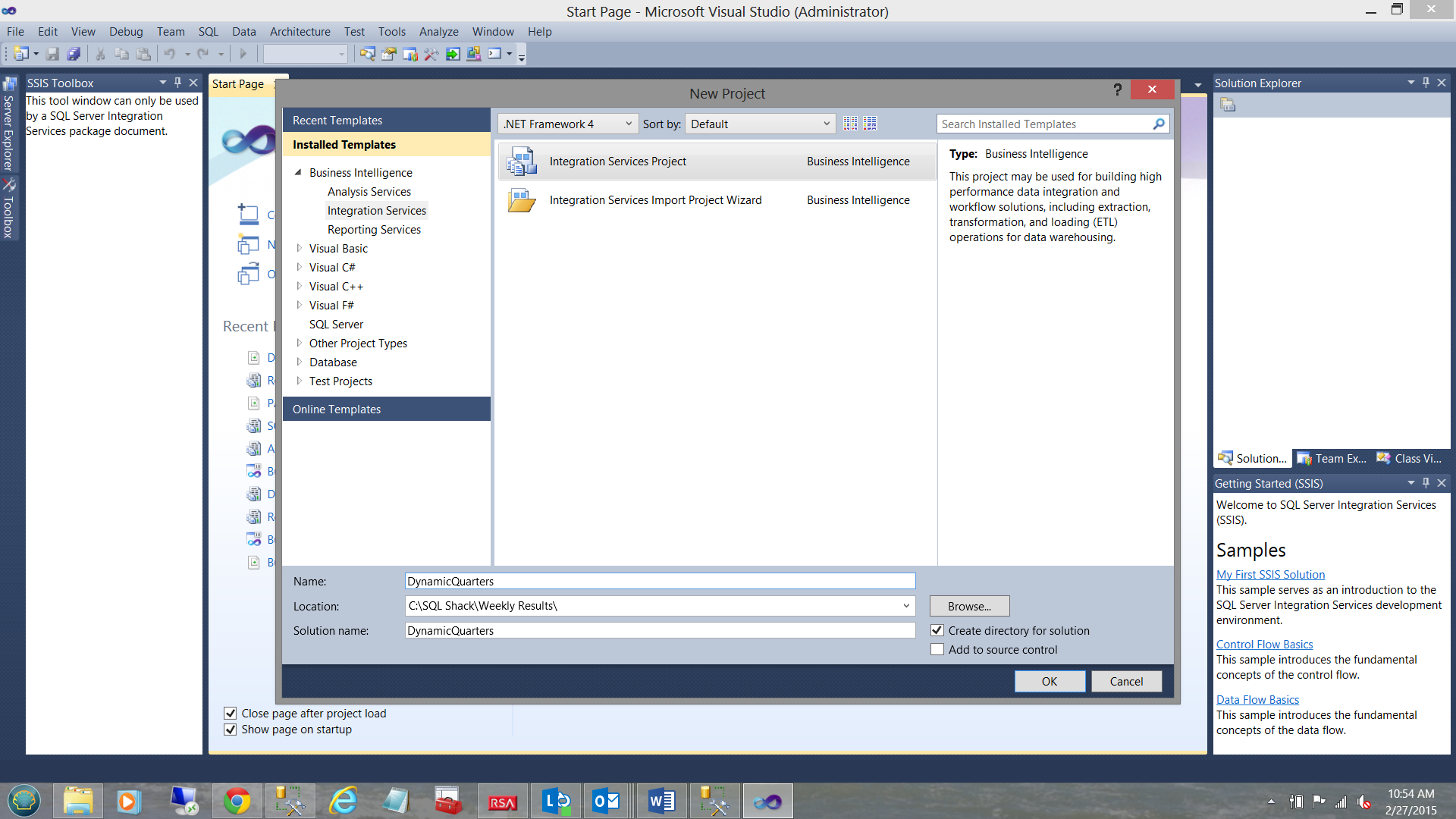
We give our project a name and click OK to create the project (see above).

我们给我们的项目起一个名字，然后单击OK创建该项目（请参见上文）。

Should you be unfamiliar with creating projects within SQL Server Data Tools do have a look at one of my other articles on SQL Shack.

如果您不熟悉在SQL Server数据工具中创建项目的话，请参阅我关于SQL Shack的其他文章之一。

We find ourselves on our working surface.

我们发现自己处于工作表面。

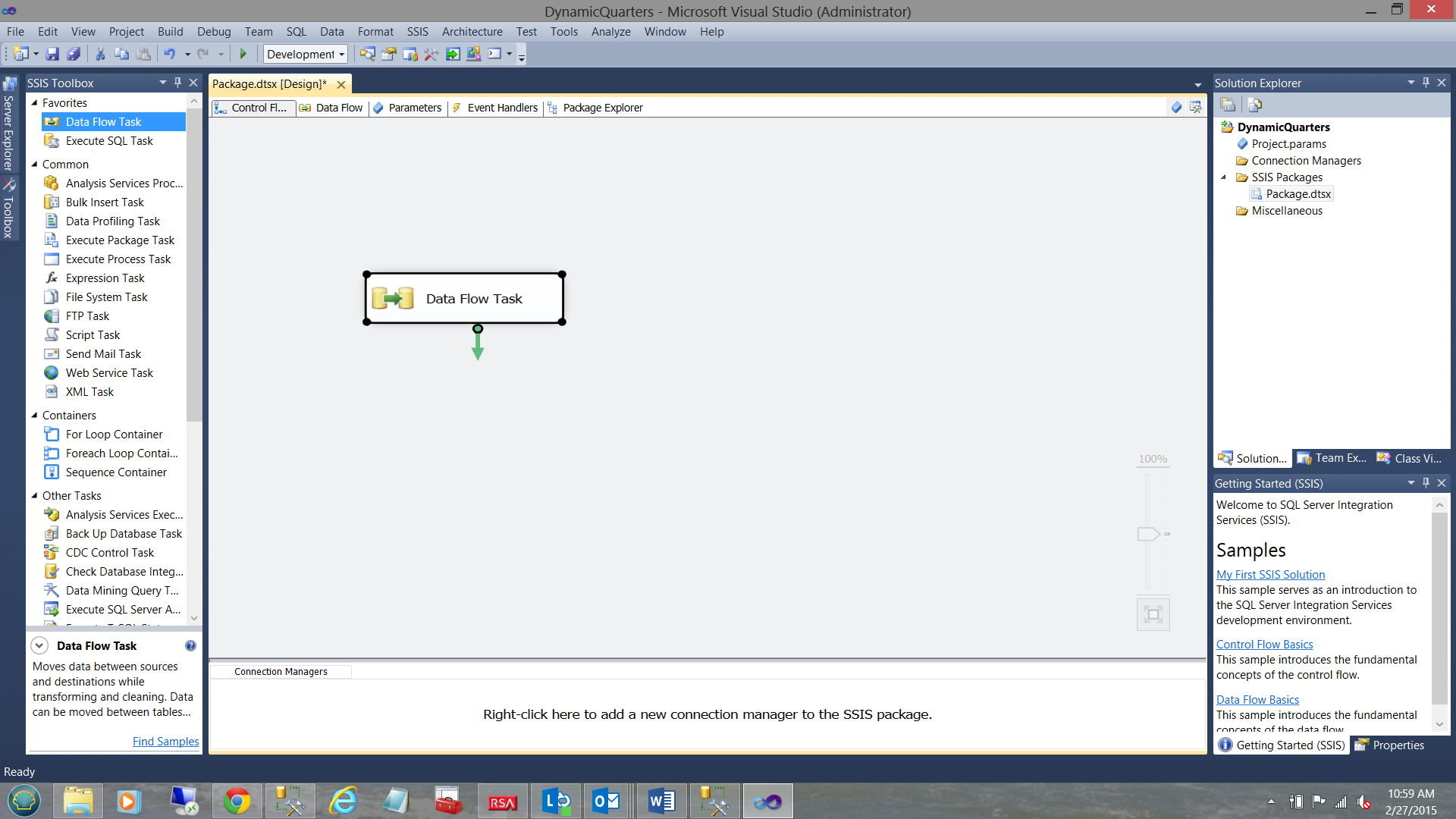
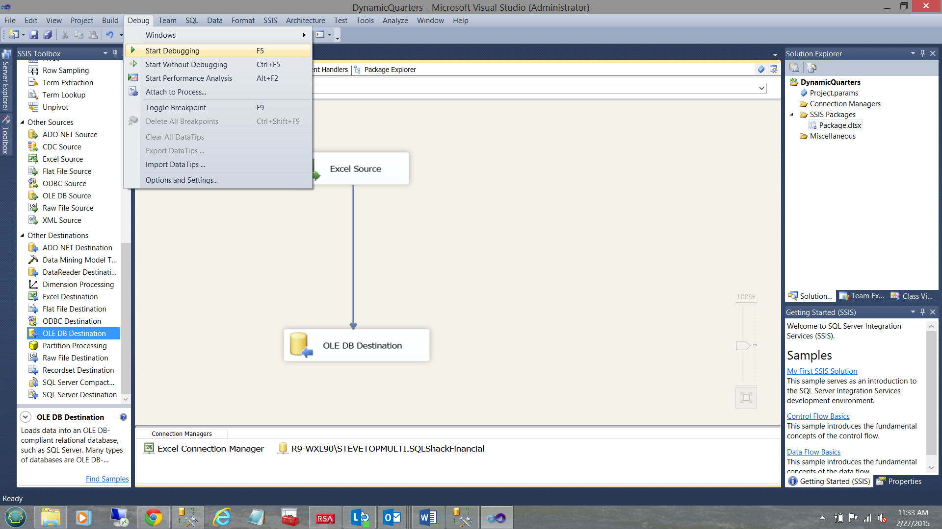
We drag a “Data Flow Task” on to our work surface as may be seen above.

如上所示，我们将“数据流任务”拖到工作面上。

Double-clicking on the “Data Flow Task” brings us to our “Data Flow Task” work surface.

双击“数据流任务”将我们带到“数据流任务”工作界面。

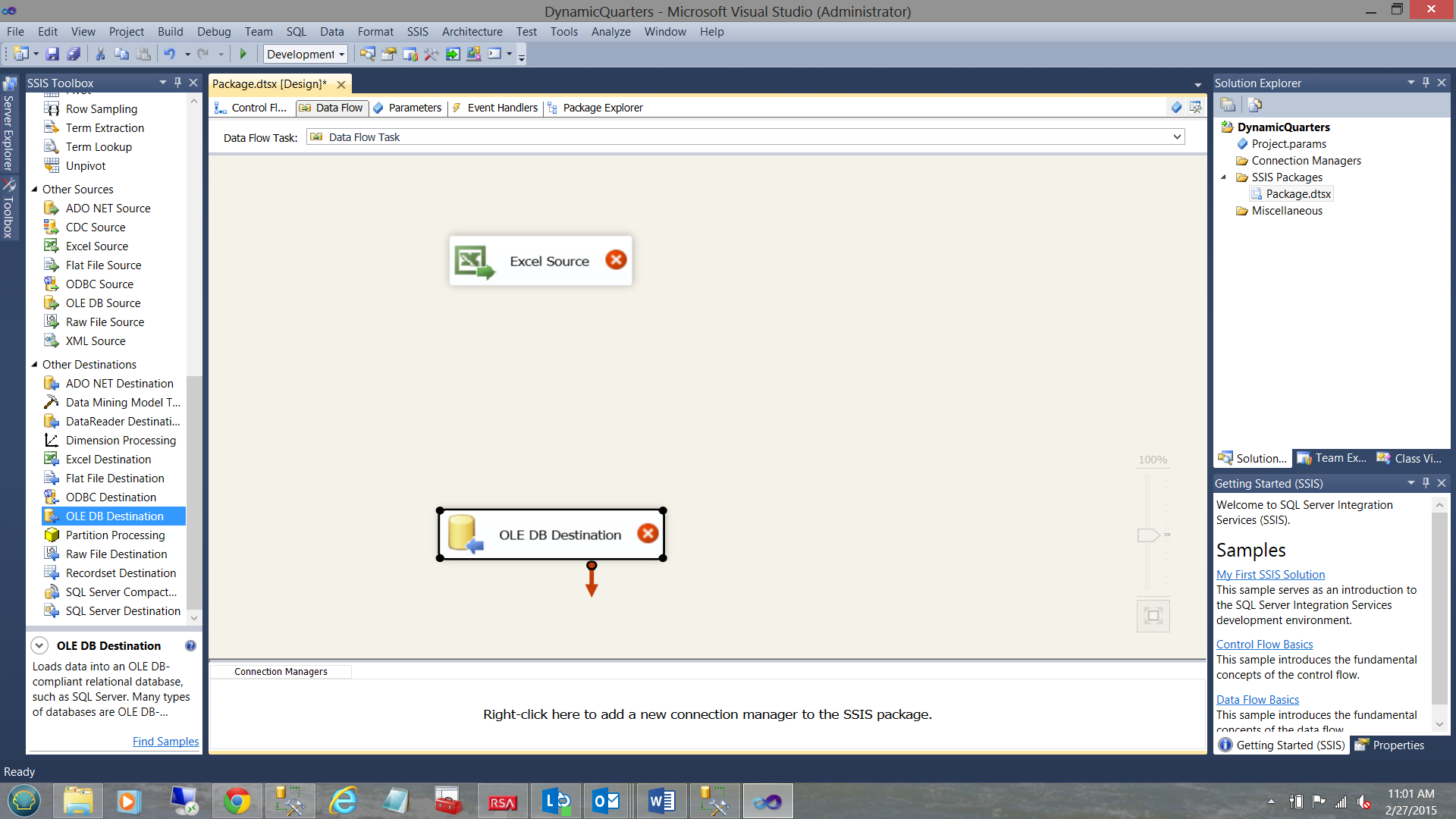
We now drag an “Excel Source” onto the work surface, in addition to an “Ole DB Destination”.

现在，除了“ Ole DB目标”之外，我们还将“ Excel Source”拖到工作面上。

We may now configure the “Excel Source”.

现在，我们可以配置“ Excel Source”。

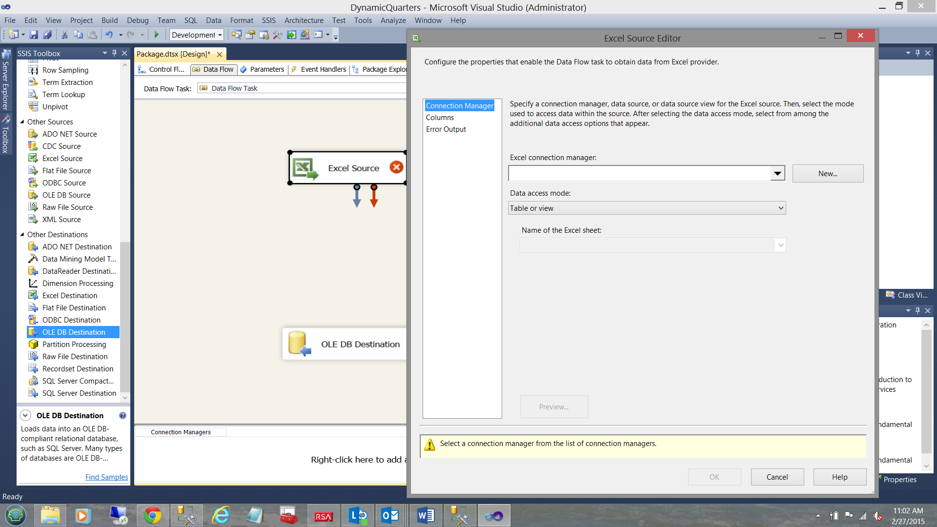
By double-clicking on the “Excel Source” the “Excel Source Editor” is brought into view. We click the “New” button (see above).

通过双击“ Excel Source”，将显示“ Excel Source Editor”。我们点击“新建”按钮（见上文）。

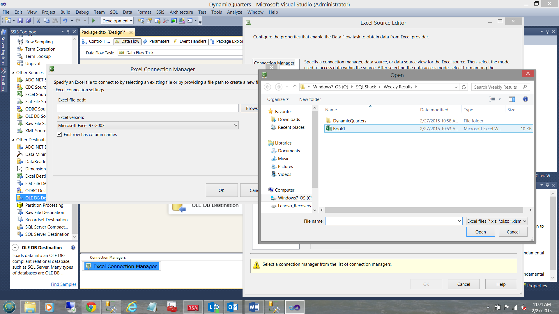
The “Excel Connection Manager” is now visible and we select the ‘Browse” button to look for our source data spreadsheet “Book1” (see above). We select “Book1” and click “Open”.

现在可以看到“ Excel Connection Manager”，并且我们选择“浏览”按钮来查找源数据电子表格“ Book1”（请参见上文）。我们选择“ Book1”，然后单击“打开”。

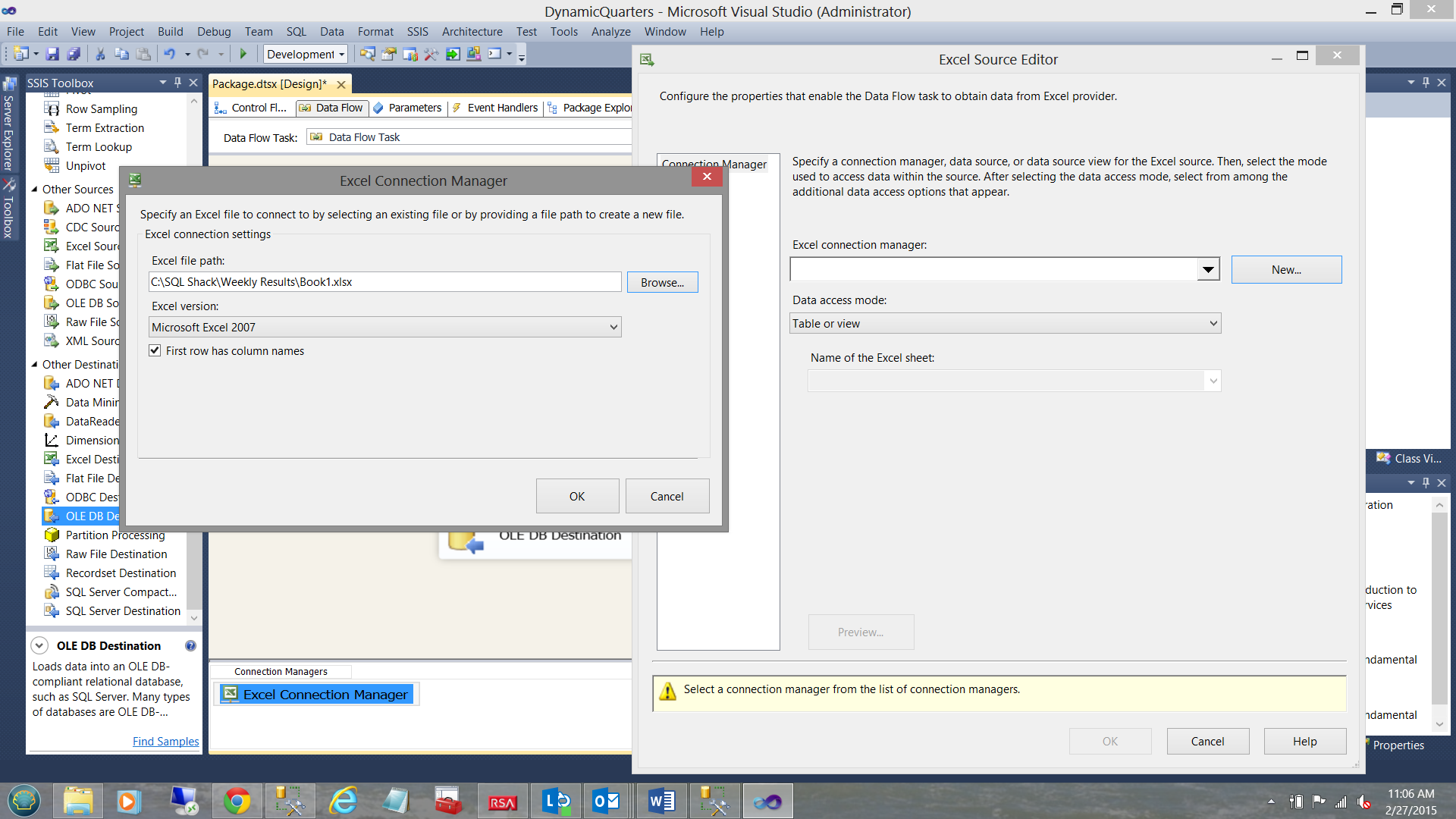
The reader will note that the spreadsheet name is visible in the “Excel Connection Manager” dialog box (see above). We click OK to leave this dialog box.

读者会注意到，电子表格名称在“ Excel Connection Manager”对话框中可见（见上文）。我们单击“确定”离开此对话框。

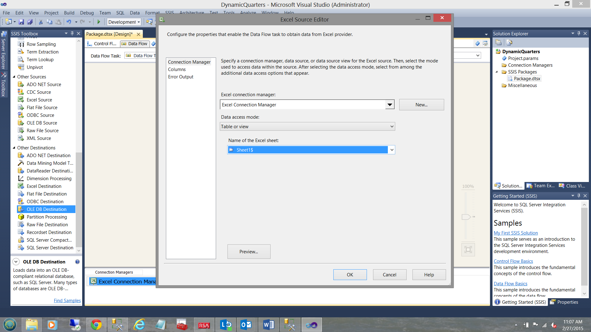
We find ourselves back in the “Excel Source Editor”. We select “Sheet1$” from the “Name of the Excel sheet” dialog box (see above).

我们发现自己回到了“ Excel Source Editor”。我们从“ Excel工作表的名称”对话框中选择“ Sheet1 $”（请参见上文）。

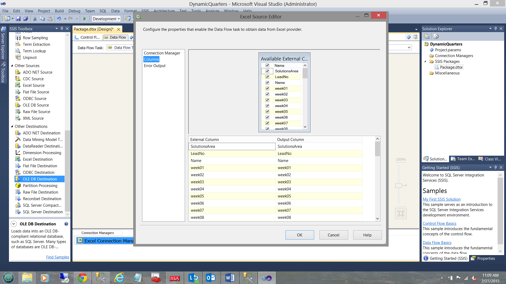
Clicking the “Columns” tab, we see the columns that are present within the spreadsheet. We click “OK” to accept what we have (see above).

单击“列”选项卡，我们将看到电子表格中存在的列。我们单击“确定”接受我们所拥有的（见上文）。

This achieved, we must now configure our data destination. This will be a table within the SQL Shack Financial database.

为此，我们现在必须配置数据目标。这将是SQL Shack Financial数据库中的表。

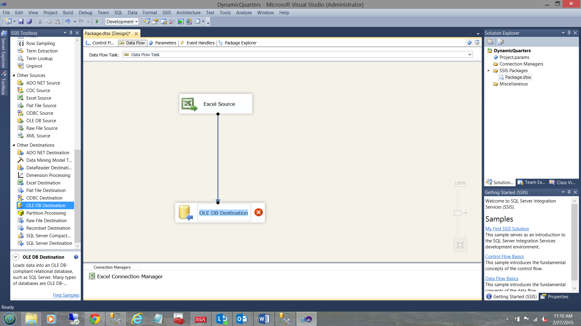
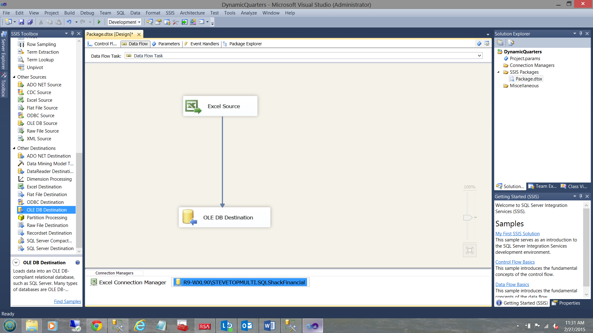
We first join the “Excel Source” to the “OLE DB Destination” (see above).

我们首先将“ Excel Source”加入“ OLE DB Destination”（请参见上文）。

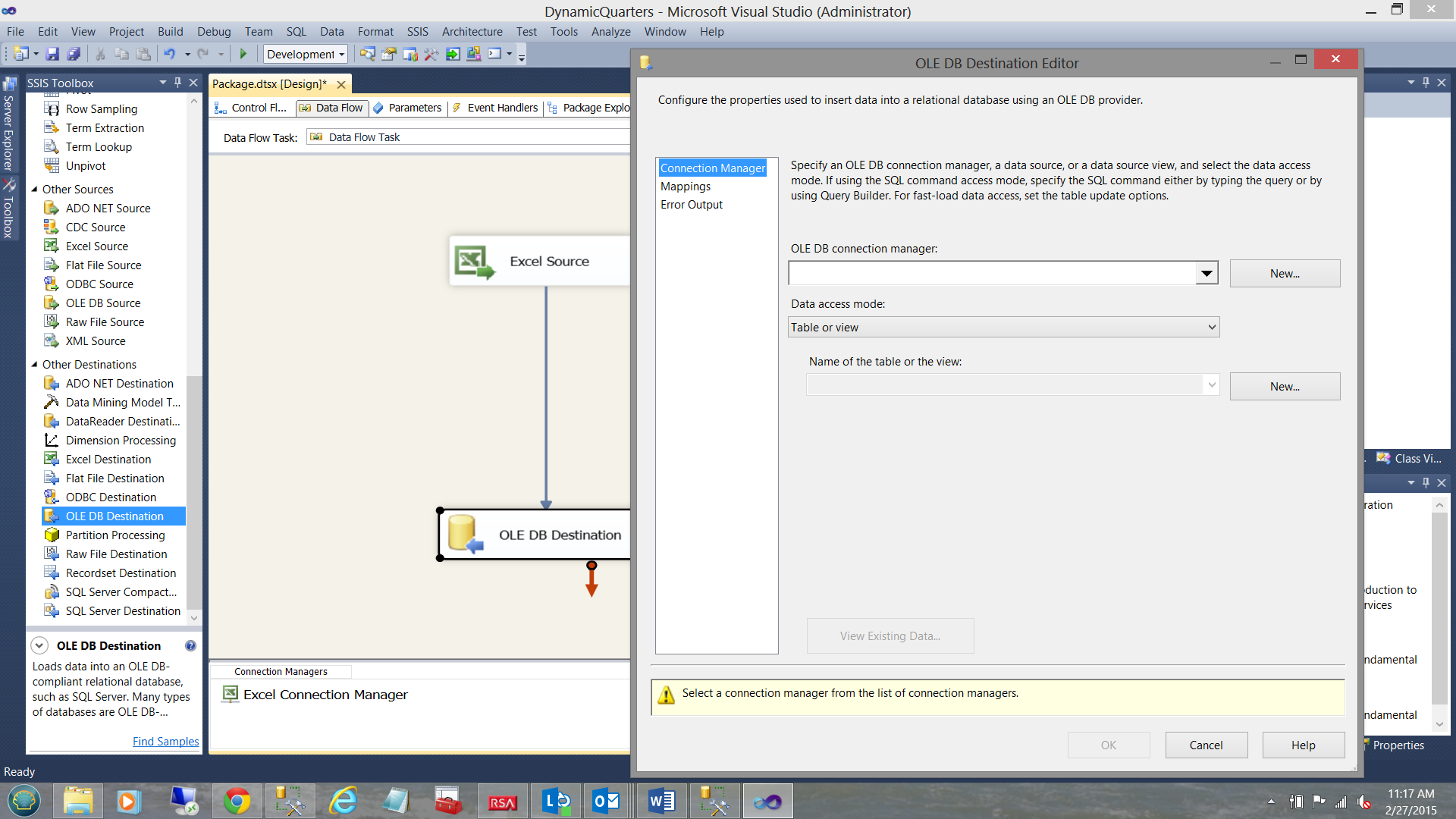
Once again, double-clicking on the “OLE DB Destination”, brings up the Editor (see above).

再次双击“ OLE DB目标”，将显示编辑器（请参见上文）。

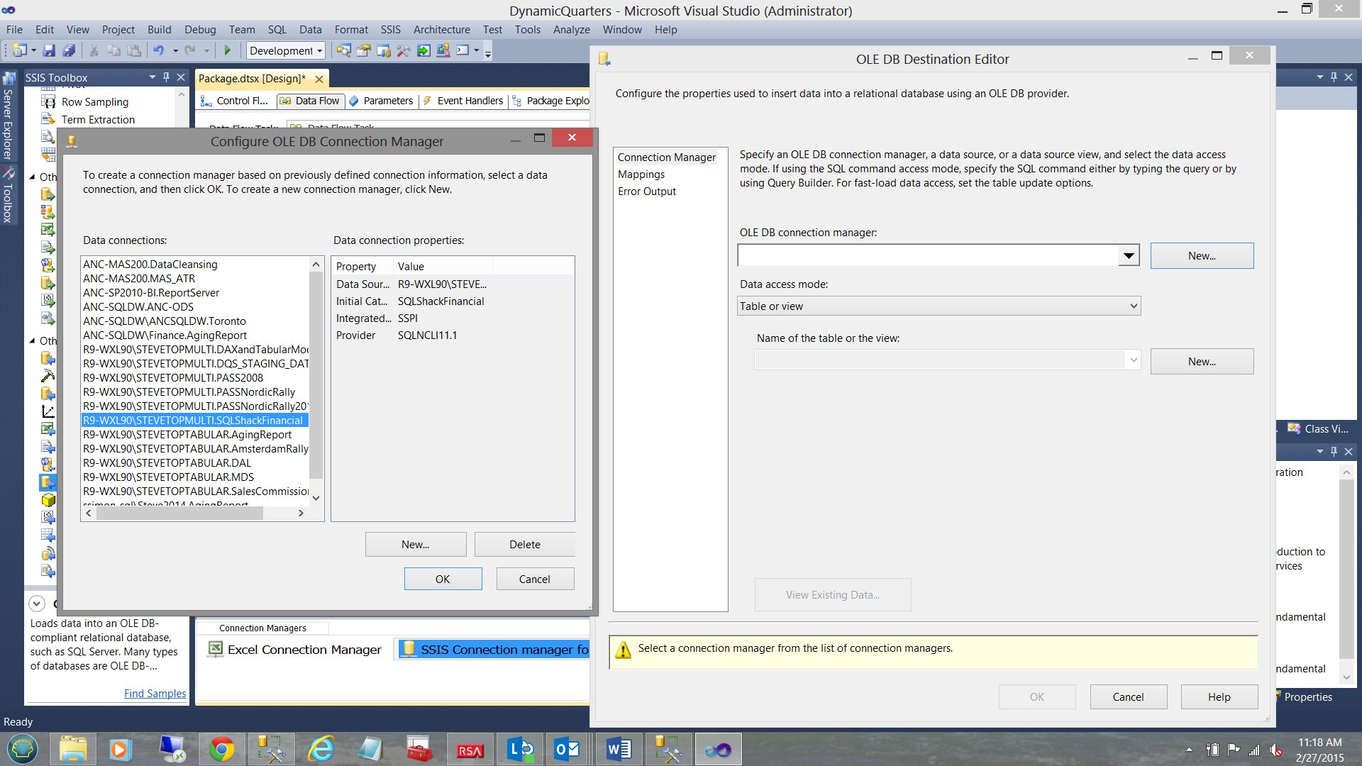
We select the “New” option by clicking the “New” button to the right of the “OLE DB connection manager” drop-down box. The “Configure OLE DB Connection Manager” dialog box is brought into view. We select the SQL Shack Financial database as may be seen highlighted above and to the left. We click “OK” to leave the “Configure OLE DB Connection Manager” dialog box and we find ourselves back in the “OLE DB Destination Editor” (see below).

我们通过单击“ OLE DB连接管理器”下拉框右侧的“新建”按钮来选择“新建”选项。进入“配置OLE DB连接管理器”对话框。我们选择了SQL Shack Financial数据库，如上方和左侧所示。我们单击“确定”离开“配置OLE DB连接管理器”对话框，然后回到“ OLE DB目标编辑器”（请参见下文）。

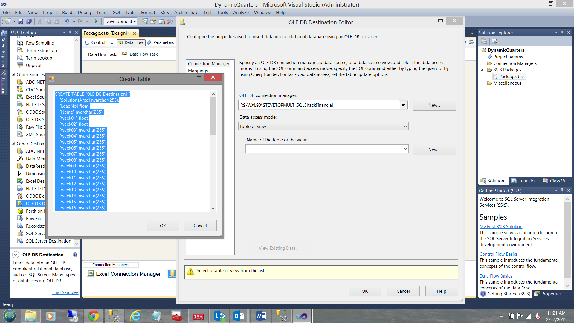
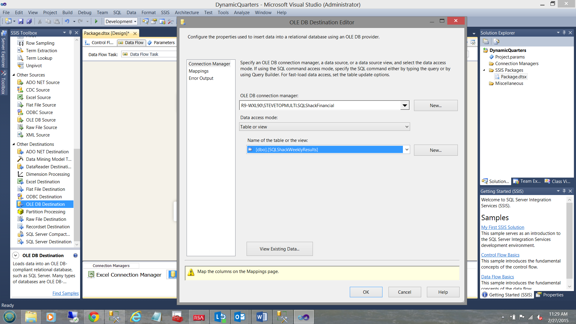
We must now create our destination table within the “SQLShackFinancial” database. We click “New” beside the “Name of the table or the view” drop-down box (see above). The “Create Table” box is brought into view. The astute reader will note that a proposed table definition is shown (see above and to the left). We shall change the proposed table name from “OLE DB Destination” to “SQLShackWeeklyResults”. We click “OK” to leave this dialogue box. The important point to remember is that when we do click “OK”, the physical table is then created within the database.

现在，我们必须在“ SQLShackFinancial”数据库中创建目标表。我们单击“表或视图的名称”下拉框旁边的“新建”（请参见上文）。将显示“创建表”框。精明的读者会注意到，其中显示了建议的表定义（请参见上方和左侧）。我们将提议的表名从“ OLE DB Destination”更改为“ SQLShackWeeklyResults”。我们单击“确定”离开此对话框。要记住的重要一点是，当我们单击“确定”时，便会在数据库中创建物理表。

The table having been created, we now are able to place that table name into the “Name of the table or the view” drop down box (see below).

创建完表格后 ，我们现在可以将该表格名称放入“表格或视图的名称”下拉框中（见下文）。

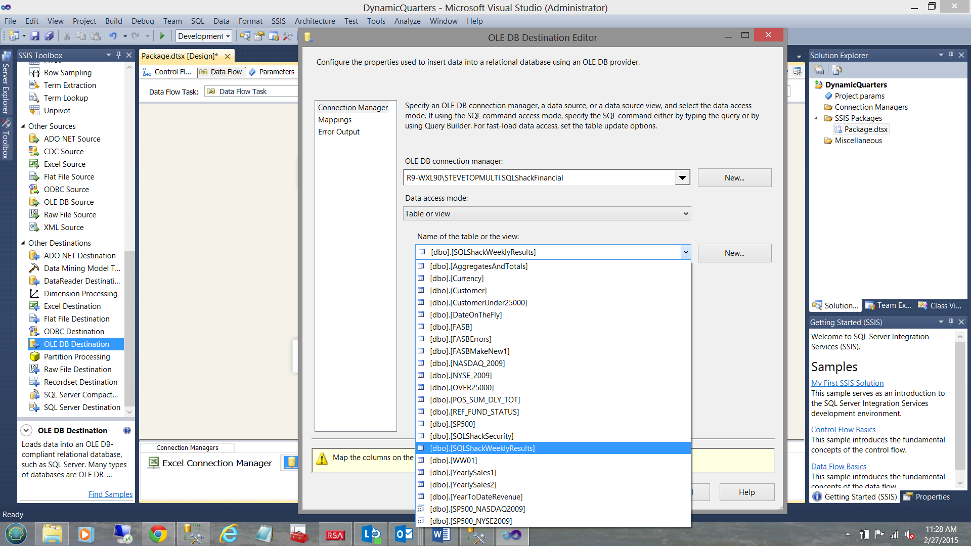
We select the table name (see above).

我们选择表名（见上文）。

Once again, we are returned to our “OLE DB Destination Editor” (see above).

再次，我们返回到“ OLE DB目标编辑器”（请参见上文）。

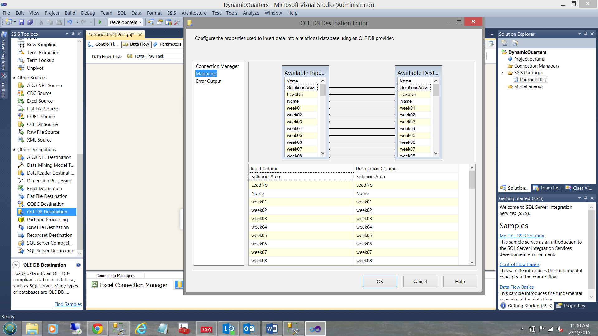
Clicking the “Mappings” tab (see above) we note the one to one mapping of the fields in the source Excel spreadsheet to the fields within the database table (see above).

单击“映射”选项卡（见上文），我们注意到源Excel电子表格中的字段与数据库表中的字段（见上文）的一对一映射。

We click “OK to leave the dialog box and find ourselves back on the drawing surface.

我们单击“确定”离开对话框，然后回到图形表面。

加载数据 ( Loading the data )

All that remains is to load our raw data from the spreadsheet that the client maintains, into our database table.

剩下的就是将客户维护的电子表格中的原始数据加载到我们的数据库表中。

We do so by clicking the “Debug” tab (as we are running the package manually). Normally the load would be scheduled utilizing the SQL Server Agent.

我们可以通过单击“调试”选项卡来实现（因为我们正在手动运行该软件包）。通常，将使用SQL Server代理计划负载。

大GOTCHA ！！！ ( The big GOTCHA!!! )

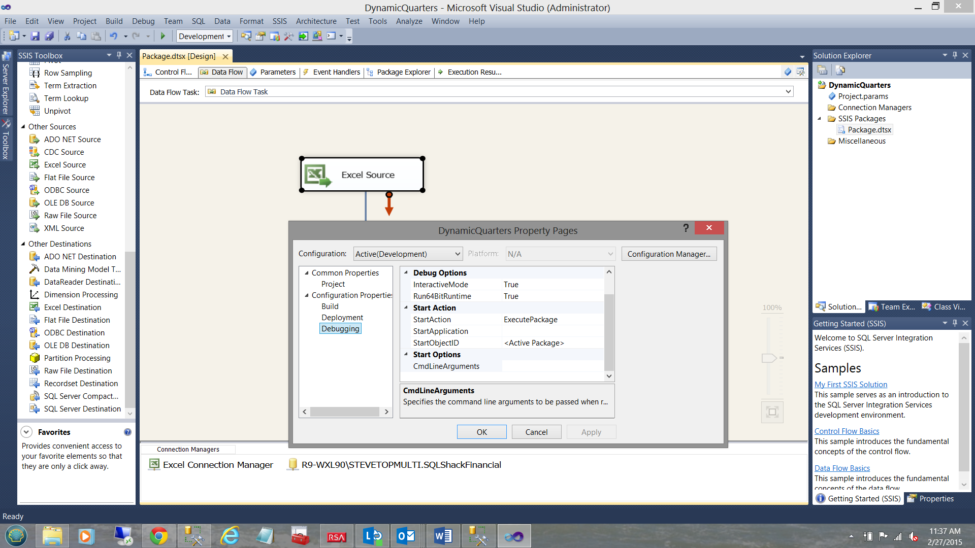
Should you be running a 32-bit installation, then the load WILL FAIL with the ugliest error message. We must first change the “Debug Option” property “Run64BitRunTime” from true to False (see above).

如果您正在运行32位安装，则加载将失败并显示最丑陋的错误消息。我们必须首先将“调试选项”属性“ Run64BitRunTime”从true更改为False（请参见上文）。

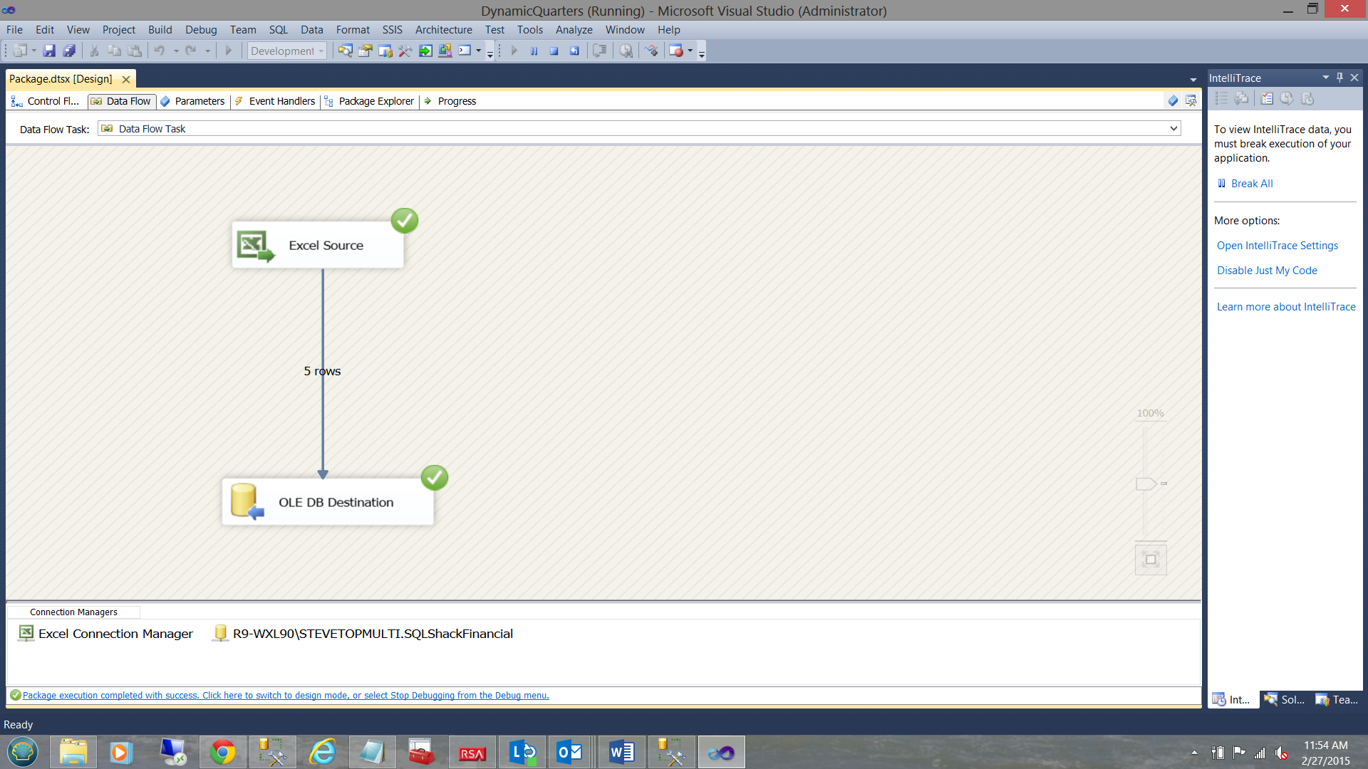
Clicking the “Debug” option and “Start Debugging” we are able to load our data into the table (see above).

单击“调试”选项和“开始调试”，我们可以将数据加载到表中（见上文）。

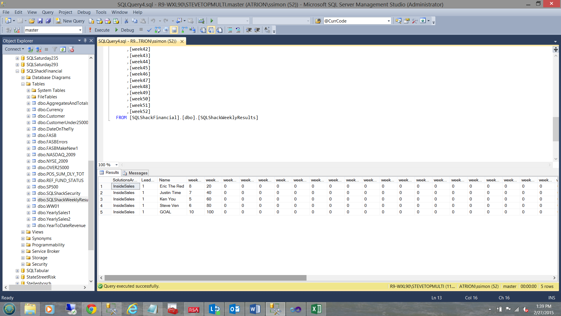
Looking at the table that we just populated within our database, we find the following (see above).

查看刚刚填充到数据库中的表，我们发现以下内容（请参见上文）。

深入骨头 ( Getting to the meat on the bone )

With the data present within the database table we are now in a position to craft our T-SQL query. The complete code listing may be found in Addenda 1.

有了数据库表中的数据，我们现在可以设计T-SQL查询了。完整的代码清单可在附录1中找到。

We begin by declaring a few variable. The reader will note that there wads of these variables and this was the most efficient however not the most effective manner in which to create the query. The total record volume would be under 10,000 and that said, including time deadlines, I opted for the “good ole quick and dirty”.

我们首先声明一些变量。读者会注意到，有一堆这些变量，这是创建查询的最有效但不是最有效的方式。总记录量将少于10,000个，也就是说，包括截止日期在内，我选择了“好又脏又好”。

Once again I have spent many years working with Oracle (which is cursor based). Although we hate these ‘animals’ there are times when they do come in handy. When your data resides in a temporary table and there is little to no chance of locking production tables, I am of the opinion that there is little risk.

我再次花了很多年与Oracle（基于游标）一起工作。尽管我们讨厌这些“动物”，但有时候它们确实派上用场。当您的数据位于临时表中并且几乎没有机会锁定生产表时，我认为风险很小。

Having declared all the necessary variables and having my data available to me, I declare a table variable called “Weekly Values”. The table variable will contain:

声明了所有必需的变量并提供了我的数据后，我声明了一个名为“每周值”的表变量。该表变量将包含：

The clients workgroup name (e.g. Inside Sales)
客户工作组名称（例如内部销售）
The lead number (an ordinary integer and not really relevant to our discussion)
主角编号（一个普通的整数，与我们的讨论无关）
The name of the employee (e.g. Steve Ven)
员工姓名（例如，史蒂夫·文（Steve Ven））
The amount of sales calls made (for that week)
那个星期的销售电话量
The number of the current week (e.g. January 5 would be week 1)
当前星期数（例如1月5日为第1周）
A sorter integer field to ensure that an imaginary person called “GOAL” is the last vertical line on the chart when we look at each week. Any other folks get a sorter value of 1.
一个排序整数字段，用于确保当我们每周查看时，一个假想的人（称为“ GOAL”）是图表上的最后一条垂直线。其他任何人得到的分拣器值为1。

光标的胆量 ( The guts of the cursor )

We open the cursor and place the value of table field “Week01” into variable @Week01 and “Week02” into variable @Week02 etc. This is achieved through “Case Logic”

我们打开光标，将表字段“ Week01”的值放入变量@ Week01，将“ Week02”放入变量@ Week02，等等。这是通过“案例逻辑”实现的

We carry a counter as we are going to loop through 52 times. The ‘eagle-eyed’ reader will tell us that any given year has approximately 52.5 weeks. To keep our chat simple, we shall assume that there are only 52 weeks in any given year. This will make more sense in a few seconds.

我们将进行52次循环，因此会携带一个计数器。 “老鹰眼”的读者会告诉我们，任何一年大约有52.5周。为了使我们的聊天简单，我们假设在任何一年中只有52周。几秒钟后，这将变得更有意义。

The case logic may been seen below:

案例逻辑如下所示：

 
Set @Weekvalue = (Select  case 
When @kounter1 = 1 then @Week01
When @kounter1 = 2 then @Week02
When @kounter1 = 3 then @Week03
When @kounter1 = 4 then @Week04
When @kounter1 = 5 then @Week05
When @kounter1 = 6 then @Week06
When @kounter1 = 7 then @Week07
--......
When @kounter1 = 51 then @Week51
When @kounter1 = 52 then @Week52 else 999 end ) 
 
INSERT @WeeklyValues VALUES (@SolutionsArea,@LeadNo,@Name,@WeekValue,@Kounter1, @sorter)
       Set @Kounter1 = @Kounter1 +1
       if @Kounter1 > 52 break

What all of this achieves is to pivot our data from the format shown in the client’s spreadsheet to a format more conducive to charting.

所有这些都是为了将我们的数据从客户电子表格中显示的格式转换为更有利于制图的格式。

Sample from the clients spreadsheet

来自客户电子表格的样本

Name	Week01	Week02	Week03
Steve Ven	10	20	30
Fred Smith	20	40	60

名称	周01	周02	周03
史蒂夫·文	10	20	30
弗雷德·史密斯	20	40	60

Format required for charting

图表所需的格式

Name	Week Number	Value
Steve Ven	1	10
Fred Smith	1	20
Steve Ven	2	20
Fred Smith	2	40
Steve Ven	3	30
Fred Smith	3	60

名称	周数	值
史蒂夫·文	1个	10
弗雷德·史密斯	1个	20
史蒂夫·文	2	20
弗雷德·史密斯	2	40
史蒂夫·文	3	30
弗雷德·史密斯	3	60

这真的如何运作？ ( How does this really work? )

The main processing occurs within the while loop (which in itself is an integral part of the cursor).

主要处理发生在while循环内（它本身是游标的组成部分）。

With the ‘current employee’, we utilize his name, the solutions area (to which he belongs), and the lead to which he was following. On the first pass through the loop, the counter has a value of 1 and therefore the value contained within the variable “Weekvalue” contains the value for the table field “Week01” (see the case logic within the code listing in Addenda1). The entire record the then written to the table variable and then the counter incremented by 1. As long as the incremented counter has not reached 53 then iteration continues with the next value being 2 (in our case). Obviously, the first part of our record retains the same solutions area, name, and lead. The only value that changes is the value of “Weekvalue”. It now takes the value of the database table field “Week02” (for THAT employee).

对于“当前雇员”，我们利用他的名字，解决方案区域（他所属的领域）以及他关注的线索。在第一次通过循环时，计数器的值为1，因此变量“ Weekvalue”中包含的值包含表字段“ Week01”的值（请参阅Addenda1代码清单中的案例逻辑）。然后将整个记录写入表变量 ，然后将计数器递增1。只要递增的计数器尚未达到53，迭代就会继续，下一个值为2（在我们的示例中）。显然，我们记录的第一部分保留了相同的解决方案区域，名称和线索。唯一更改的值是“ Weekvalue”的值。现在，它采用数据库表字段“ Week02”的值（ 对于THAT employee ）。

Once the counter has reached 53, we break from the loop and we find ourselves back in the main “fetch” of the cursor. The next employee is then obtained and so the cycle continues until we run out of employees.

一旦计数器达到53，我们就跳出循环，发现自己回到了游标的主要“读取”位置。然后获得下一位员工，因此循环继续进行，直到我们用完所有员工为止。

At the end of the process we transfer the contents of the table variable to a temporary table (#rawdata33). The reason that we do so is to ensure persistence of the result set, in case a “GO” statement (or the like) is encountered further down the code listing. As we know, a “GO” statement by nature assumes that you are finished with the table variable and thus is one of the Gotcha’s you wish to avoid.

在该过程结束时，我们将表变量的内容传输到临时表（＃rawdata33）中 。我们这样做的原因是为了确保结果集的持久性，以防在代码清单的下方遇到“ GO”语句（或类似内容）。众所周知，“ GO”语句本质上假设您已经完成了表变量的操作，因此是您希望避免的Gotcha之一。

It should be clearly understood that the same processing could have been achieved by utilizing two while loops. In most cases this is preferable, as we normally avoid the use of a cursor.

应该清楚地理解，通过利用两个while循环可以完成相同的处理。 在大多数情况下，这是可取的 ， 因为我们 通常 避免使用游标。

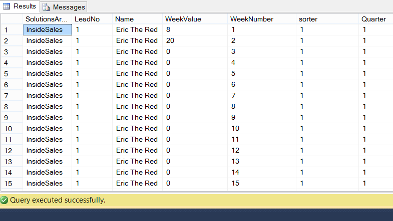
The “eagle-eyed” reader will have noted that in many of the screen dumps (that I have shown thus far), a variable called “@Sorter is displayed. A value of 1 is assigned to each “real” employee and a value of 99 is assigned to a dummy employee called “GOAL”. The goal is not really an employee but will be utilized in our reporting to show the enterprises total goals for any particular week. Thus when we look at our weekly results, we should see the following: Note the employees, the last one being “GOAL”

“老鹰眼”的读者会注意到，在许多屏幕转储中（我到目前为止已经显示过），都会显示一个名为“ @Sorter”的变量。将值1分配给每个“实际”雇员，将值99分配给一个称为“目标”的虚拟雇员。目标不是真正的员工，但将在我们的报告中用于显示企业在任何特定星期的总体目标。因此，当我们查看每周的结果时，我们应该看到以下内容：注意员工，最后一个是“目标”

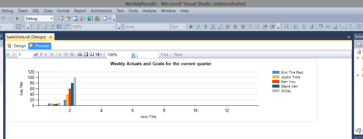
Note the grey bar to the right of the chart showing the enterprise goal. It appears to the right, as within the report we have set the sorting (for each week) to sort by @sorter ascending. More on this when we construct our report.

请注意显示企业目标的图表右侧的灰色条。它显示在右侧，因为在报告中，我们已将排序（每周）设置为按@sorter升序排序。我们在构建报告时会对此进行更多介绍。

创建我们的最终客户报告 ( Creating our end client reports )

As we can understand when it comes to reporting, report “real estate” is always problematic. This was the case when I created the first report for our end client. The report was just “to busy” and nothing could be gleaned without utilizing a magnifying glass.

正如我们所了解的那样，报告“房地产”始终是有问题的。当我为最终客户创建第一个报告时就是这种情况。该报告只是“忙碌”，不使用放大镜就无法收集任何信息。

This said we decided to show only data from the current quarter (as determined by the SQL Server Getdate() function) within our report.

这表示我们决定在报告中仅显示当前季度的数据（由SQL Server Getdate（）函数确定）。

In order to achieve this, we must alter our data extraction query to only pull data from the current quarter.

为了实现这一点，我们必须更改数据提取查询以仅从当前季度提取数据。

 
set @Yearr = (select convert(varchar(4),convert(date,Getdate())))

We first ascertain which year we are in. In our case, this will be 2015 and as such we utilize the “datepart” function to extract the current year (see above).

我们首先确定我们所在的年份。在我们的情况下，这将是2015年，因此我们利用“ datepart”功能提取当前年份（请参见上文）。

This achieved, we are in a position to define the “quarter” that we shall show to the end client and once again, this will depend upon the quarter in which the current date is found. As an example February 28^th will fall in quarter 1. I would see weekly results from January 1^st through February 28^th. Had this been the 28^th of May, then the results would have been from April 1^st through May 28^th^.

实现这一目标后，我们便可以定义要向最终客户显示的“季度”，这将再次取决于当前日期所在的季度。例如，2月28 ^日将落在第一季度。我会看到从1月1 ^日到2月28 ^日的每周结果。如果这是5月28 ^日，那么结果应该是从4月1 ^日到5月28 ^日 ^。

 
Set @Quarter =
        (case when convert(date,GetDate()) between Convert(date,@Yearr +'0101') and  Convert(date,@Yearr +'0331') then 
        '1 and 13'
         when convert(date,GetDate()) between Convert(date,@Yearr +'0401') and  Convert(date,@Yearr +'0630') then '14 and 26'
         when convert(date,GetDate()) between Convert(date,@Yearr +'0701') and  Convert(Date,@Yearr +'0930') then '27 and 39' 
         else '40 and 52' end)

The code above, helps us achieve this.

上面的代码可帮助我们实现这一目标。

Note that @quarter has been defined as Varchar(50). In the case that the current date falls within the first quarter, then the value that will be set for @quarter will be ‘1 and 13’.

请注意，@ quarter已定义为Varchar（50）。如果当前日期在第一季度之内，则将为@quarter设置的值将为“ 1和13”。

 
select a.*  into #rawdata34 
From(
select rd33.* , 
   (case when convert(date,GetDate()) between Convert(date,@Yearr +'0101') and  Convert(date,@Yearr +'0331') then 1
         when convert(date,GetDate()) between Convert(date,@Yearr +'0401') and  Convert(date,@Yearr +'0630') then 2
         when convert(date,GetDate()) between Convert(date,@Yearr +'0701') and  Convert(Date,@Yearr +'0930') then 3 else 4 end) as Quarter
 from #rawdata33 rd33)a

The code above is a bit complex. Let us have a look at the code in green. What is happening is that we are taking all the fields from the temporary table “#rawdata33” (discussed above) and adding one last field. This field which I call “quarter” not to be confused with the variable “@quarter”.

上面的代码有点复杂。让我们看看绿色的代码。发生的是，我们正在从临时表“＃rawdata33”（如上所述）中获取所有字段，并添加最后一个字段。我将此字段称为“ quarter”，不要将其与变量“ @quarter”相混淆。

The code in green would generate an extract similar to the one shown below:

绿色代码将生成类似于以下所示的摘录：

This achieved, we now place the result set into another temporary table (#rawdata34), the reason for doing so will become evident within a few seconds (see the code in red below).

为此，我们现在将结果集放置到另一个临时表（＃rawdata34）中，这样做的原因将在几秒钟内变得显而易见（请参见下面的红色代码）。

 
select a.*  into #rawdata34 
From(
select rd33.* , 
   (case when convert(date,GetDate()) between Convert(date,@Yearr +'0101') and  Convert(date,@Yearr +'0331') then 1
         when convert(date,GetDate()) between Convert(date,@Yearr +'0401') and  Convert(date,@Yearr +'0630') then 2
         when convert(date,GetDate()) between Convert(date,@Yearr +'0701') and  Convert(Date,@Yearr +'0930') then 3 else 4 end) as Quarter
 from #rawdata33 rd33
)a

Our next task is to define one last variable @NSQL defined as a NVARCHAR(2000). We construct the following SQL Statement and place the “string” into our @NSQL variable(see below).

我们的下一个任务是将最后一个变量@NSQL定义为NVARCHAR（2000）。我们构造以下SQL语句，并将“字符串”放入我们的@NSQL变量中（请参见下文）。

 
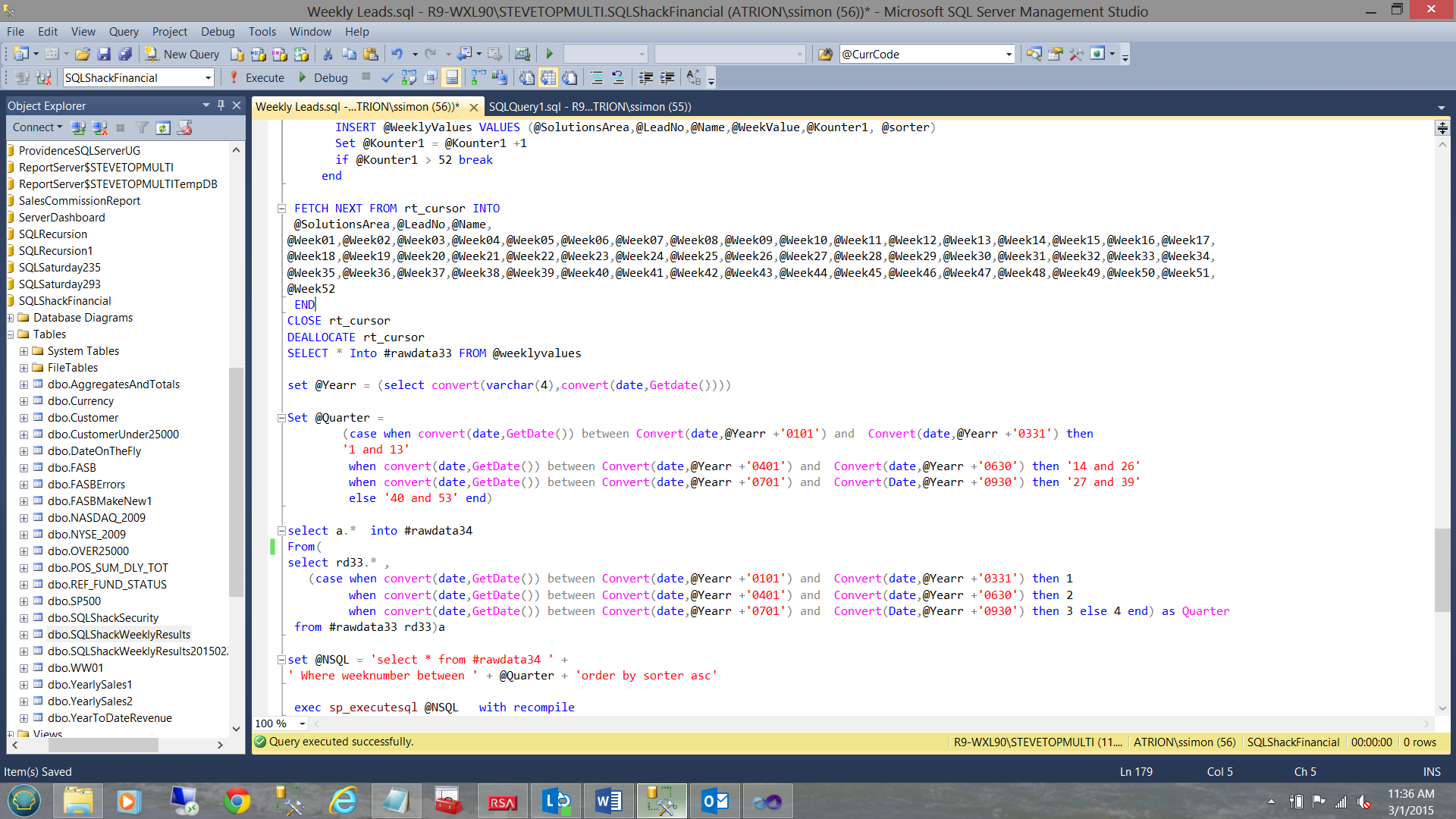
 set @NSQL = 'select * from #rawdata34 ' +
' Where weeknumber between ' + @Quarter + 'order by sorter asc'

The reason behind this madness is to be able to execute THIS statement ( i.e. @NSQL ) at run time (see below).

这种疯狂的原因是能够 在运行时 执行 THIS 语句（ 即@NSQL ） （请参见下文）。

 
  exec sp_executesql @NSQL   with recompile

The end result will be that from the original records, only the records from the first quarter will be extracted.

最终结果将是从原始记录中仅提取第一季度的记录。

创建必要的用户报告 ( Creating the necessary user report )

Opening SQL Server Development Tools we create a Reporting Services project.

打开SQL Server开发工具，我们创建一个Reporting Services项目。

As we have done in past, we create our “Shared Data Source”.

与过去一样，我们创建了“共享数据源”。

Should you be unfamiliar with creating projects, creating data source connections and datasets (within SQL Server Reporting Services), do have a look at my article entitled “Now you see it, now you don’t” /now-see-now-dont/ where the process is described in detail.

如果您不熟悉创建项目，创建数据源连接和数据集（在SQL Server Reporting Services中），请看看我的标题为“现在您看到了，现在您不知道了”的文章/ now-see-now-dont / ，其中详细描述了该过程。

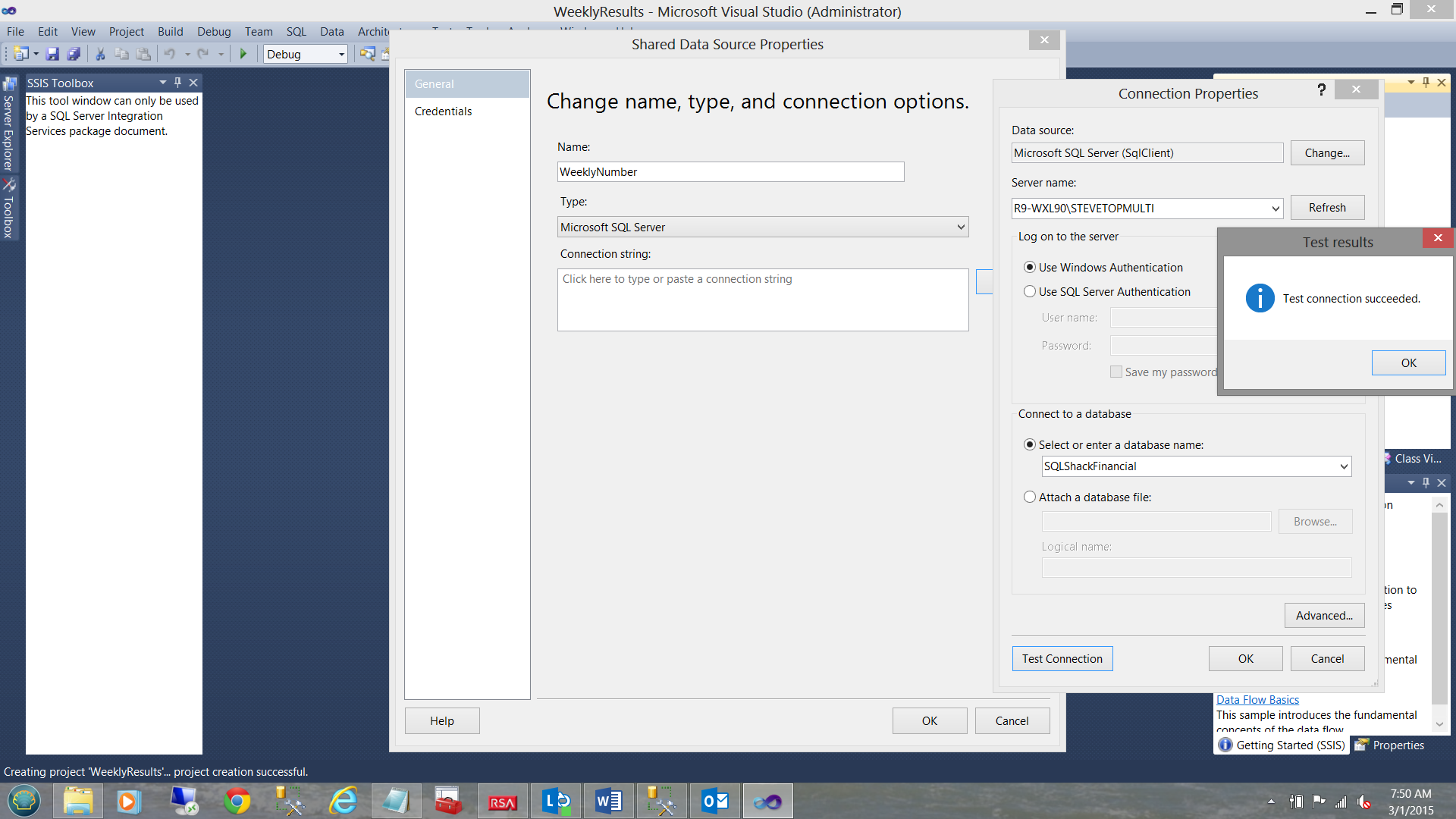
We create our shared data source called “WeeklyNumber” and point this to our SQLShackFinancial database (see above).

我们创建名为“ WeeklyNumber”的共享数据源，并将其指向我们SQLShackFinancial数据库（请参见上文）。

Having created our “Shared Data Source” we now create our first and only report.

创建了“共享数据源”之后，我们现在创建第一个也是唯一的报告。

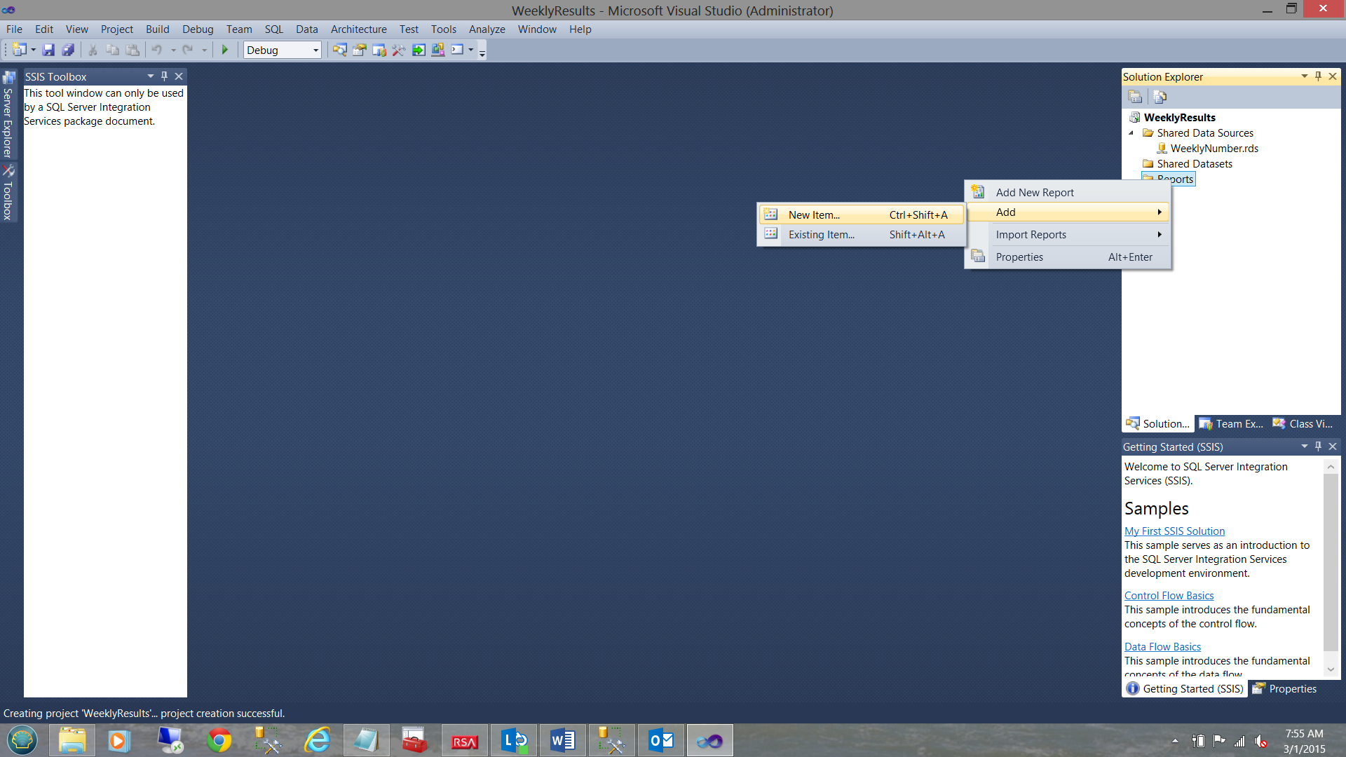
We right-click upon our report folder and select “Add” and “New Item” (from the context menu). See above.

我们右键单击报告文件夹，然后选择“添加”和“新建项”（从上下文菜单中）。往上看。

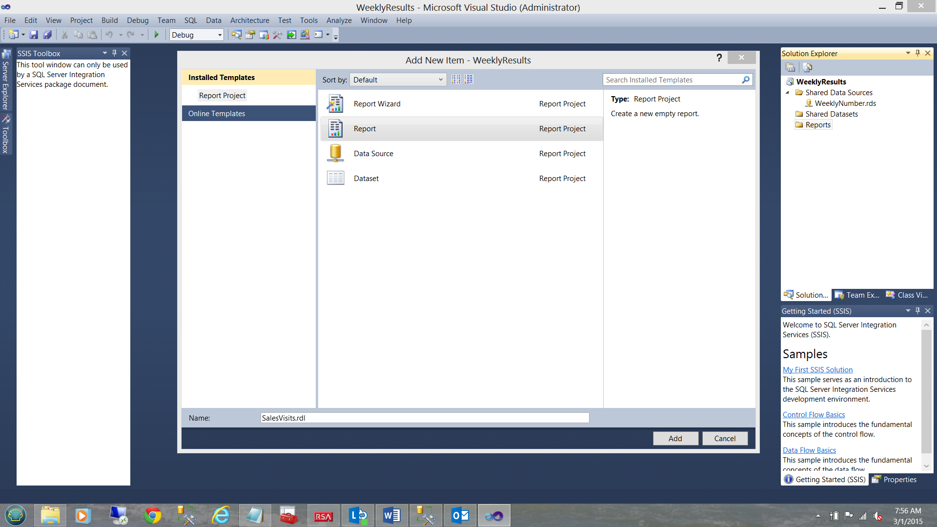
We select “Report” from the “Add New Item” menu (see above and to the middle). We give our report the name “SalesVisits”. We click “Add”.

我们从“添加新项”菜单中选择“报告”（请参见上方和中间）。我们将报告命名为“ SalesVisits”。我们点击“添加”。

Our report work surface is brought up (see above).

我们的报告工作界面被调出（见上文）。

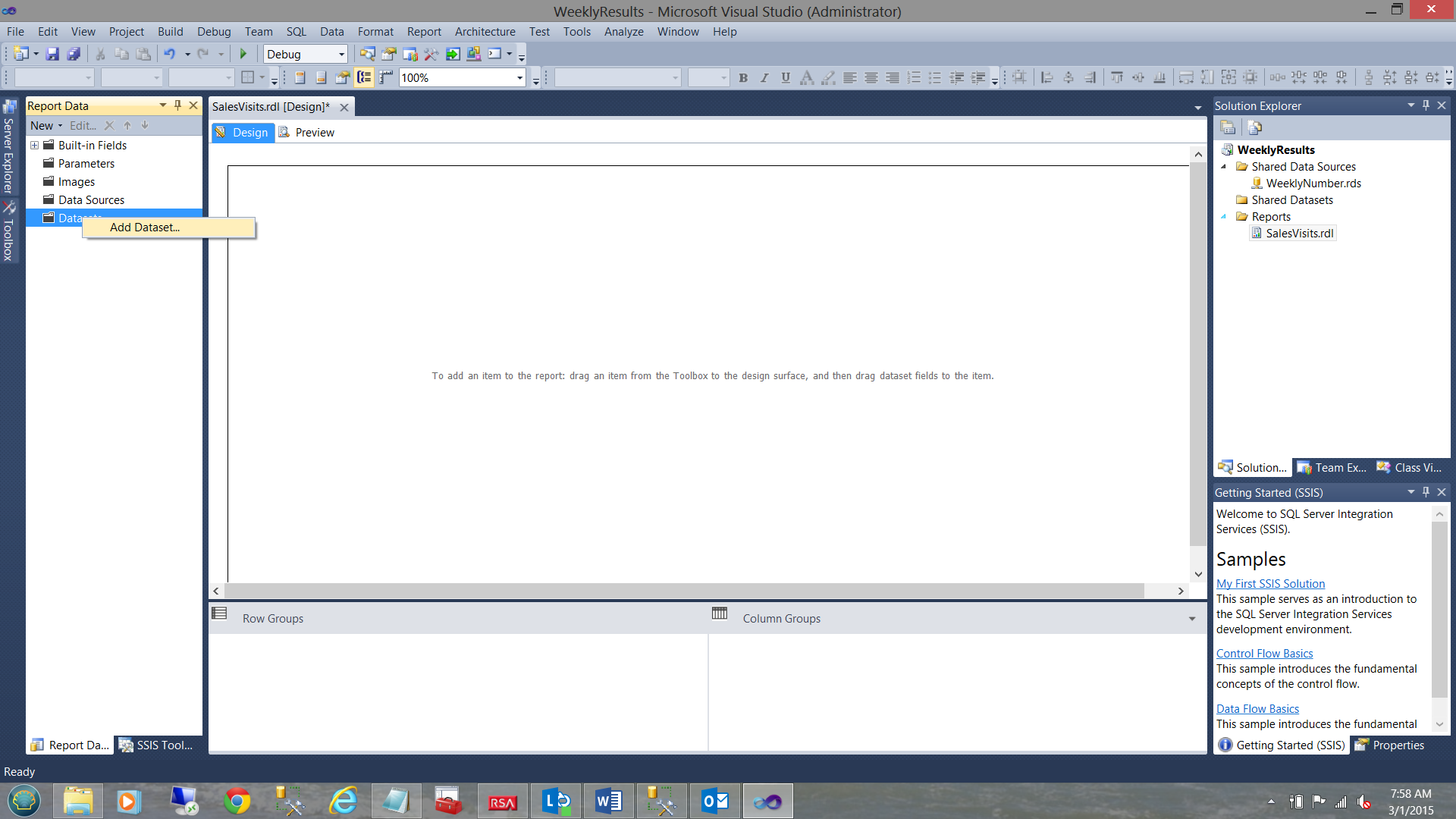
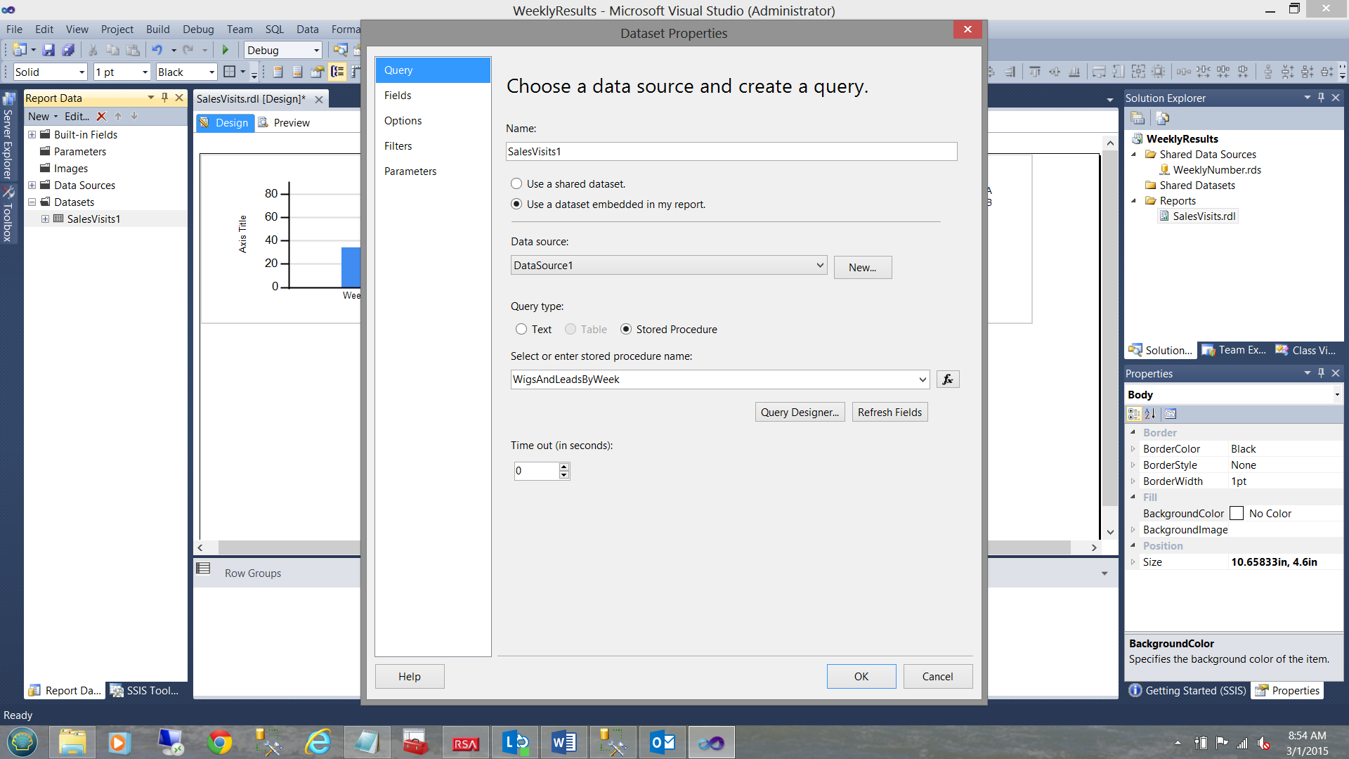
We now add a dataset by right-clicking on the “Dataset” folder and selecting “Add Dataset” from the context menu (see above).

现在，我们通过右键单击“ Dataset”文件夹并从上下文菜单中选择“ Add Dataset”来添加数据集（请参见上文）。

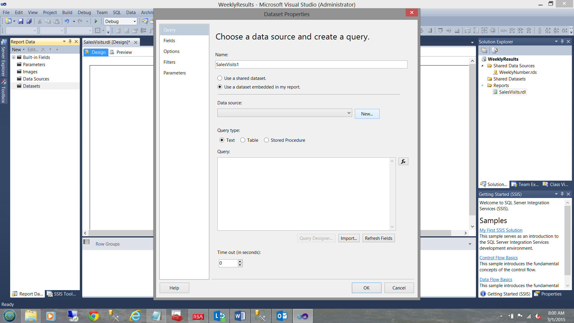
We find ourselves within the “Dataset Properties” dialogue box. We give our dataset the name “SalesVisits1”. We also select the “Use a dataset embedded in my report” option (see above). We click the “New” button to the right of the “Data source” drop down to create an “embedded” or local data source.

我们在“数据集属性”对话框中找到自己。我们将数据集命名为“ SalesVisits1”。我们还选择“使用报表中嵌入的数据集”选项（请参见上文）。我们单击“数据源”右侧的“新建”按钮，以创建“嵌入式”或本地数据源。

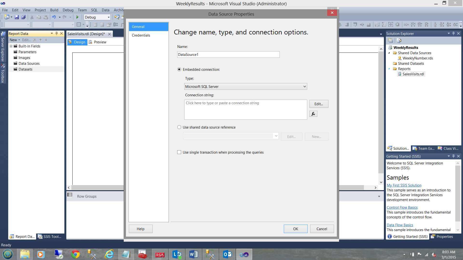
The “Data Source Properties” dialogue box is presented to us (see above).

向我们显示了“数据源属性”对话框（请参见上文）。

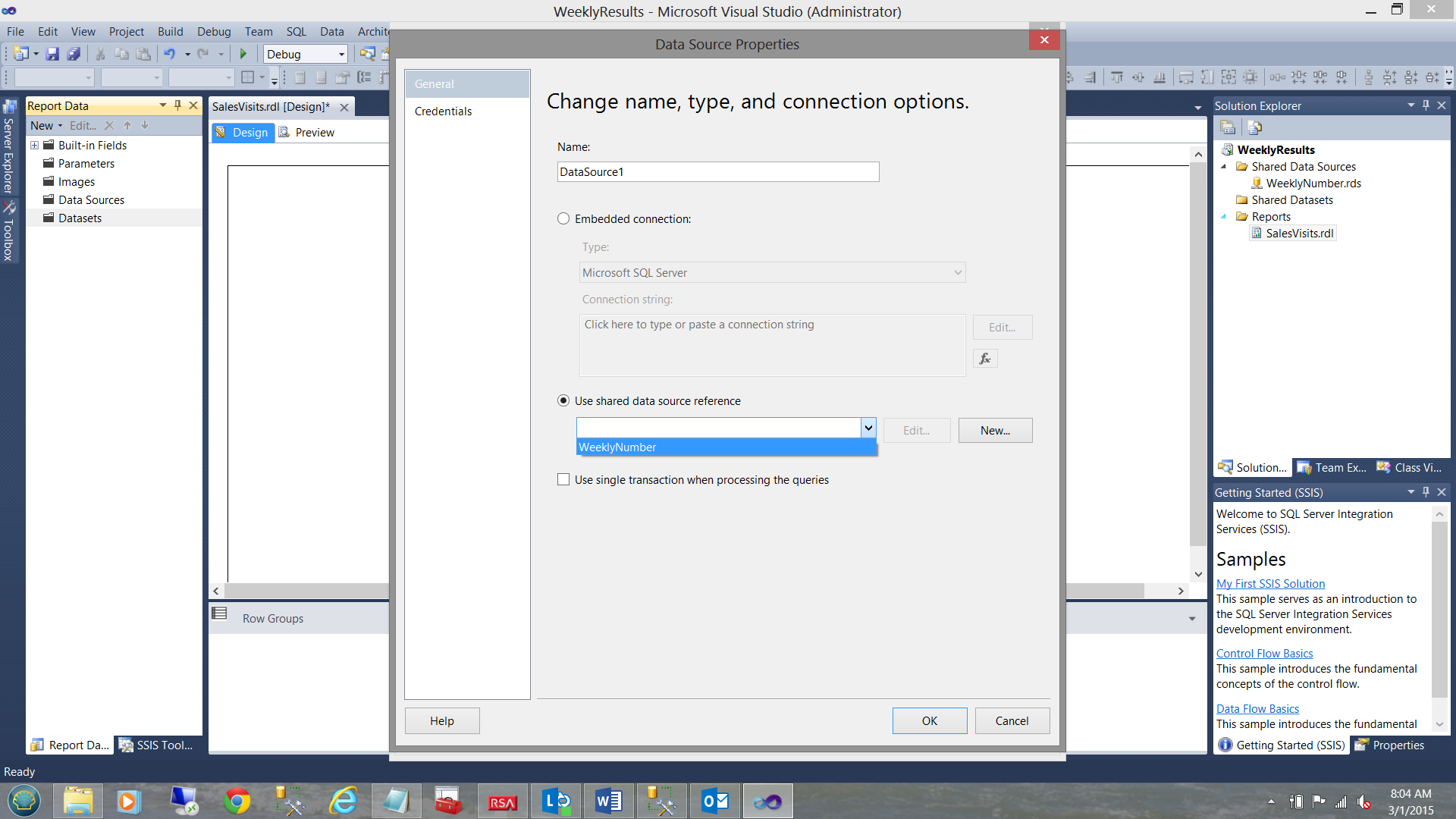
We opt to use the “Shared data source” that we created above (see the screenshot above). We click “OK” to accept our shared data source.

我们选择使用上面创建的“共享数据源”（请参见上面的屏幕截图）。我们单击“确定”接受我们的共享数据源。

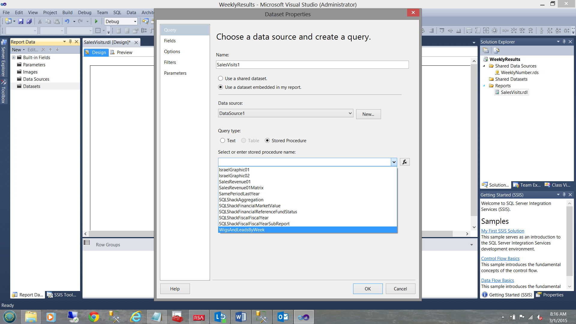
We find ourselves back on the “Dataset Properties” window. We select the stored procedure called “WigsAndLeadsByWeek” which is the name that I gave to the stored procedure that I created from the query that we have been discussing above (see the screenshot above). We click “OK” to leave this window.

我们回到“数据集属性”窗口。我们选择名为“ WigsAndLeadsByWeek”的存储过程，这是我为根据上面已经讨论过的查询创建的存储过程指定的名称（请参见上面的屏幕截图）。我们单击“确定”离开该窗口。

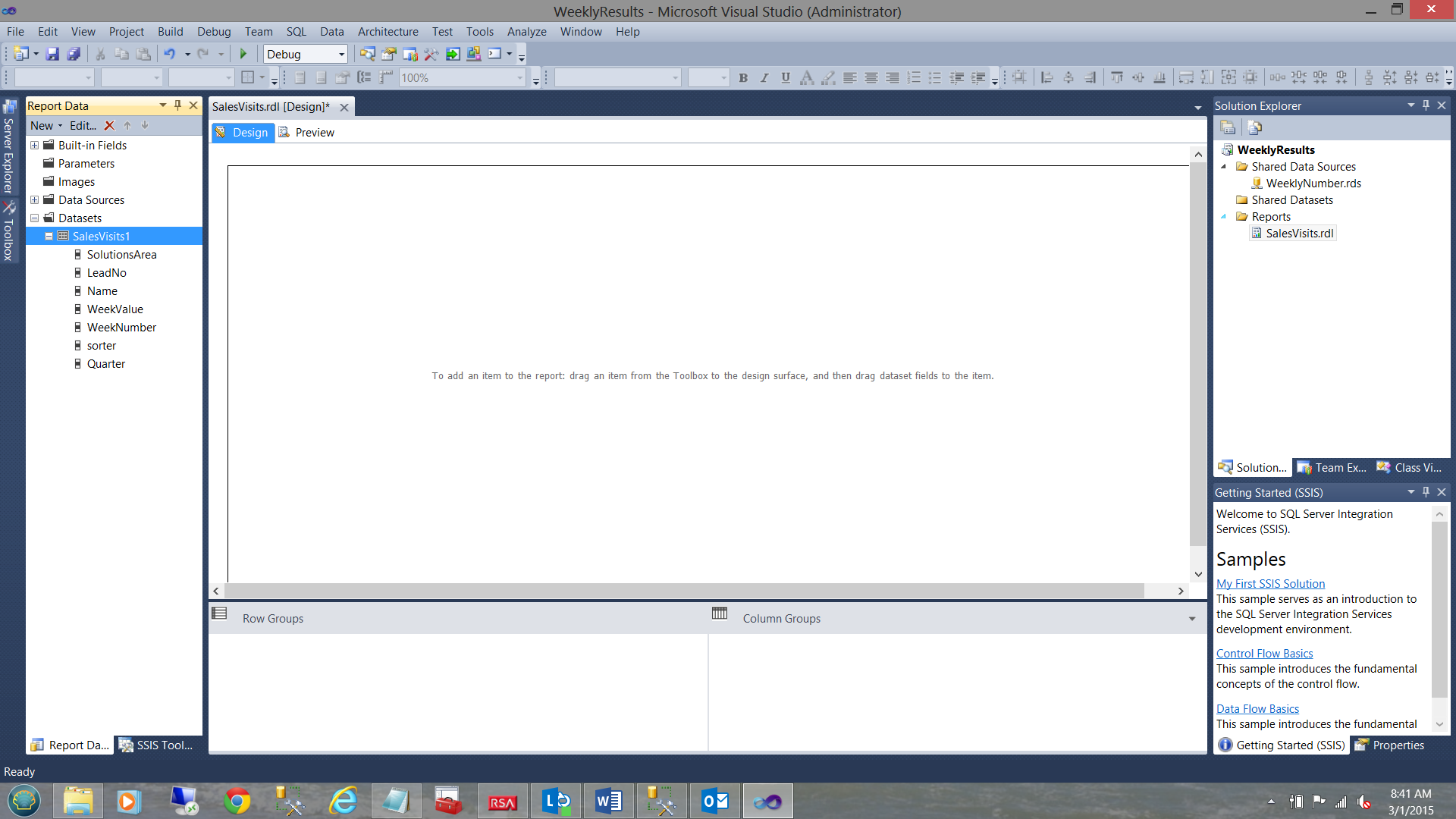
We find ourselves back on our report surface.

我们发现自己回到了报告的表面。

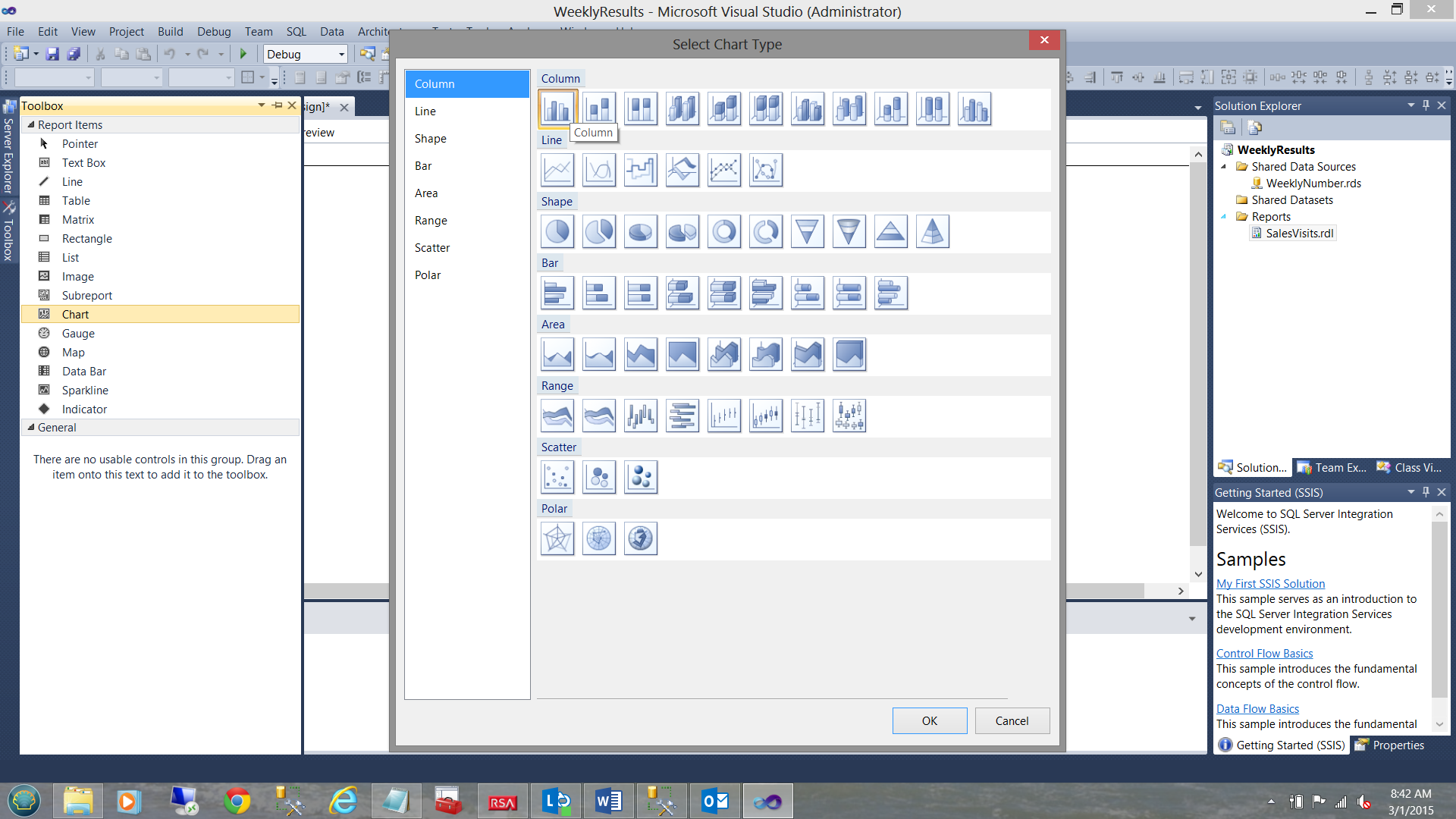
From our toolbox, we select a vertical bar chart to place upon our drawing surface (see above).

从工具箱中，我们选择一个垂直条形图放置在我们的绘图表面上（见上文）。

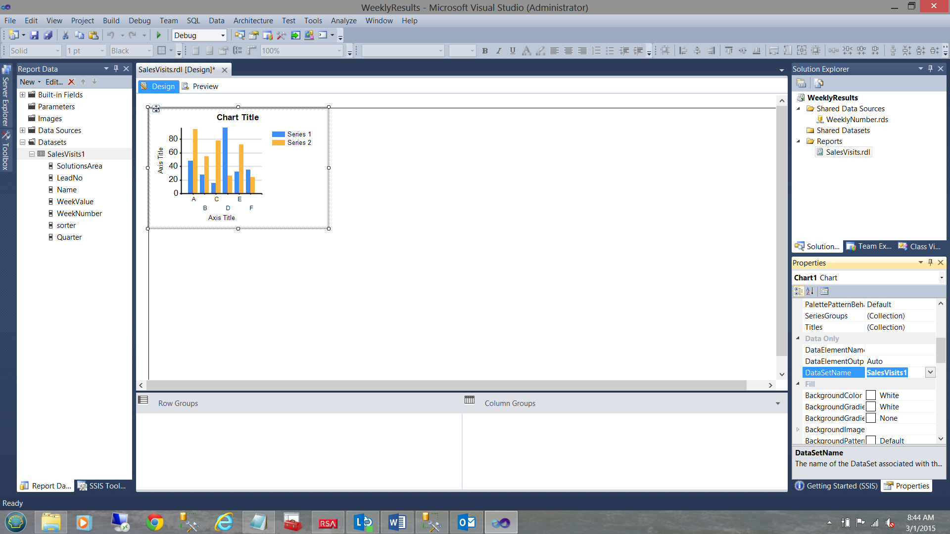
We note that the bar chart now appears upon our drawing surface. Within the properties window, we set the “DataSetName” property (of the chart) to the name of the dataset that we have just created (see above).

我们注意到，条形图现在出现在我们的绘图表面上。在属性窗口中，将（图表的）“ DataSetName”属性设置为刚刚创建的数据集的名称（请参见上文）。

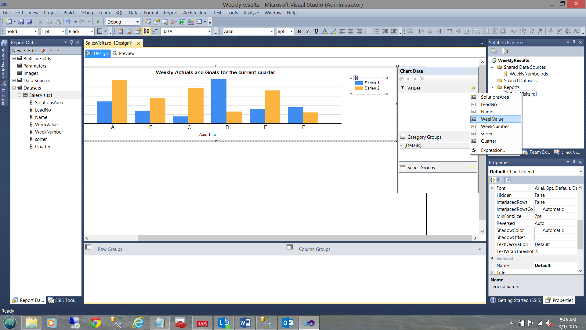
Expanding our chart and giving it a title, we are now in a position to assign the chart data.

扩展图表并为其命名，现在我们可以分配图表数据。

We set the ∑ values to “WeekValue” (see above).

我们将∑值设置为“ WeekValue”（请参见上文）。

The “Category Groups” are set to the week number (see above).

“类别组”设置为星期数（请参见上文）。

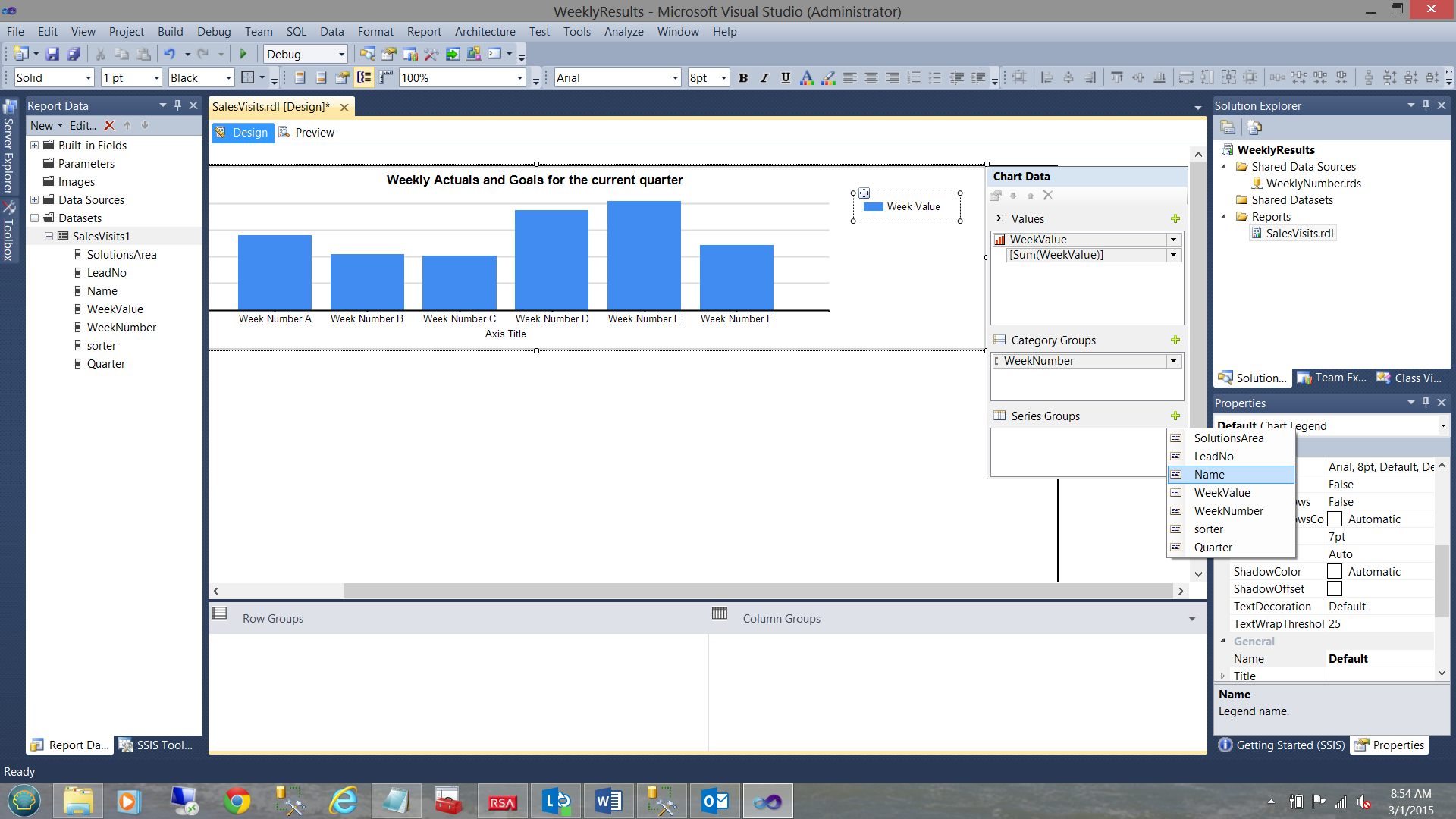
The “Series Group’’ is set to “Name” (i.e. employee names).

“系列组”设置为“名称”（即员工姓名）。

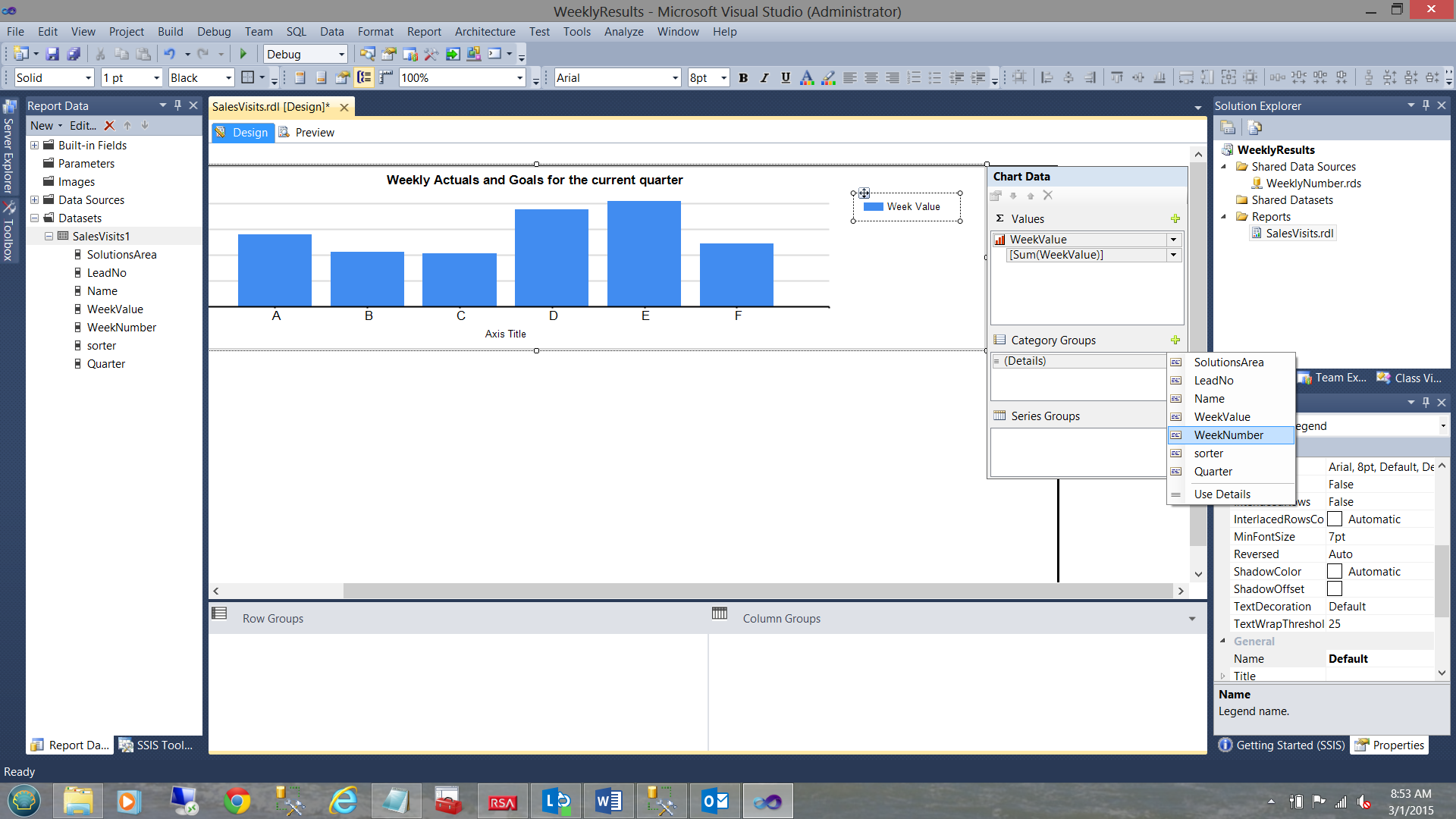
Opening our dataset once again we are going to set a few filters. The reason for this is because while this example is a simple one, the client planned to use the same dataset for other solutions areas and other lead numbers. This way our dataset is generic.

再次打开数据集，我们将设置一些过滤器。这样做的原因是，尽管此示例很简单，但客户计划将相同的数据集用于其他解决方案领域和其他潜在客户编号。这样我们的数据集是通用的。

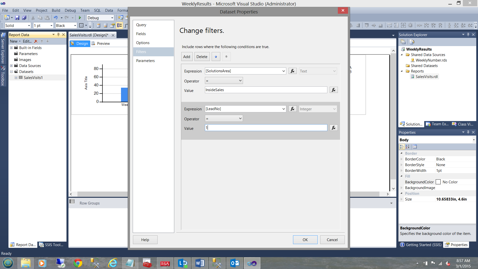
We set our solutions area to “InsideSales” and our lead number to a value of 1 (see above).

我们将解决方案区域设置为“ InsideSales”，而潜在客户数设置为1（请参见上文）。

嘿！！那么我们谈到的@sorter变量呢？ ( Hey!! What about the @sorter variable about which we spoke )

Our final task is to ensure that when the results are displayed that, the “GOAL” is shown as the last vertical bar (for each week that is displayed).

我们的最终任务是确保在显示结果时，“目标”显示为最后一个竖线（对于显示的每个星期）。

To ensure this happens, we right click upon “Names Series” grouping (see below).

为了确保这种情况发生，我们右键单击“名称系列”分组（请参见下文）。

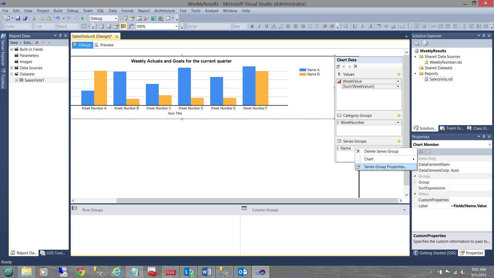
We note that the context menu is brought up. We select “Series Group Properties” (see above).

我们注意到弹出了上下文菜单。我们选择“系列组属性”（见上文）。

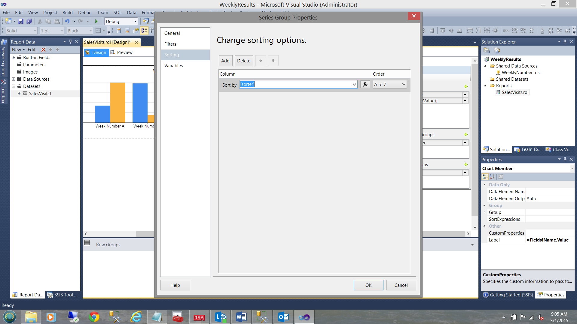
The “Series Group Properties” Dialog box is brought into view. We change the “Sort by” field to our “sorter” field (see above). We ensure that the “Order” drop-down is set to “A to Z”.

将显示“系列组属性”对话框。我们将“排序依据”字段更改为“分类”字段（请参见上文）。我们确保将“订单”下拉列表设置为“ A到Z”。

This will ensure that the sorter “99” associated with “GOAL” records will be the last name for each week (see above). We click “OK” to leave this dialogue box.

这将确保与“目标”记录关联的分类器“ 99”将成为每周的姓氏（请参见上文）。我们单击“确定”离开此对话框。

让我们试一下吧！ ( Let us give it a run! )

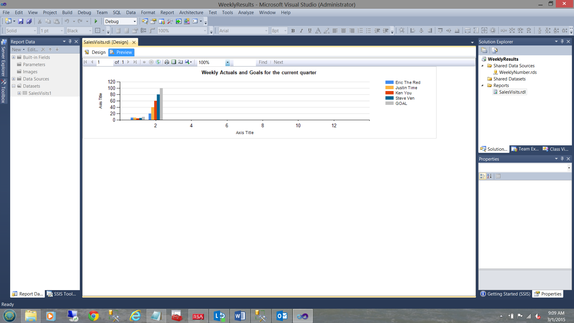
Clicking on the “Preview” tab, we are able to see the results. In our case, the reader will note that the corporate goals are grey in color and they are in fact the last vertical bar for each week.

单击“预览”选项卡，我们可以看到结果。在我们的案例中，读者会注意到公司目标是灰色的，实际上它们是每周的最后一个竖线。

结论 ( Conclusions )

Thus we have achieved our end goal of converting the format of data (which was not conducive to being utilized with a vertical bar chart) into a dataset which would enable us to produce valuable corporate information.

因此，我们达到了将数据格式（不利于垂直条形图使用）转换为数据集的最终目标，这将使我们能够产生有价值的公司信息。

User resistance to change is not the exception but rather the rule. We often have to massage data prior to getting it into a usable format. In our case, this was an end user, addicted to utilizing a spreadsheet and in a format that he or she felt comfortable using.

用户对变更的抵制不是例外，而是规则。在将数据转换为可用格式之前，我们经常必须对数据进行按摩。在我们的案例中，这是一个最终用户，他沉迷于使用电子表格并以他或她感到舒适的格式使用。

Finally, it is important (as most people will tell you) to think outside of the box and to be able to convert end user-generated challenges into productive and functional solutions.

最后，重要的是（正如大多数人会告诉您的那样）跳出思路，将最终用户产生的挑战转化为生产性和功能性的解决方案。

As a reminder, all the code used within the query may be found in the code listing in Addenda 1.

提醒一下，查询中使用的所有代码都可以在附录1的代码清单中找到。

Also please remember that should you wish to obtain a copy of the Reporting Services project do contact me.

另外请记住，如果您希望获得Reporting Services项目的副本，请与我联系。

In the interim, happy programming!!

在此期间，编程愉快！！

附录1 ( Addenda 1 )

 
use [SQLShackFinancial]
go
 
IF OBJECT_ID(N'tempdb..#rawdata1') IS NOT NULL
BEGIN
     DROP TABLE #rawdata1
END
IF OBJECT_ID(N'tempdb..#rawdata33') IS NOT NULL
BEGIN
     DROP TABLE #rawdata33
END
 IF OBJECT_ID(N'tempdb..#rawdata34') IS NOT NULL
BEGIN
     DROP TABLE #rawdata34
END
IF OBJECT_ID(N'tempdb..#rawdata55') IS NOT NULL
BEGIN
     DROP TABLE #rawdata55
END
go
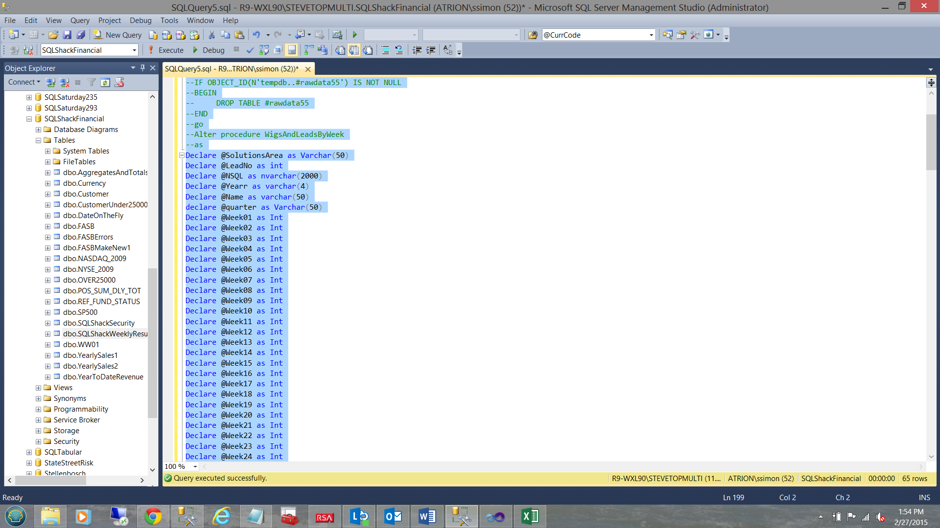
Alter procedure WigsAndLeadsByWeek
as
Declare @SolutionsArea as Varchar(50)
Declare @LeadNo	as int
Declare @NSQL as nvarchar(2000)
Declare @Yearr as varchar(4)
Declare @Name as varchar(50)
declare @quarter as Varchar(50)
Declare @Week01 as Int
Declare @Week02 as Int
Declare @Week03 as Int
Declare @Week04 as Int
Declare @Week05 as Int
Declare @Week06 as Int
Declare @Week07 as Int
Declare @Week08 as Int
Declare @Week09 as Int
Declare @Week10 as Int
Declare @Week11 as Int
Declare @Week12 as Int
Declare @Week13 as Int
Declare @Week14 as Int
Declare @Week15 as Int
Declare @Week16 as Int
Declare @Week17 as Int
Declare @Week18 as Int
Declare @Week19 as Int
Declare @Week20 as Int
Declare @Week21 as Int
Declare @Week22 as Int
Declare @Week23 as Int
Declare @Week24 as Int
Declare @Week25 as Int
Declare @Week26 as Int
Declare @Week27 as Int
Declare @Week28 as Int
Declare @Week29 as Int
Declare @Week30 as Int
Declare @Week31 as Int
Declare @Week32 as Int
Declare @Week33 as Int
Declare @Week34 as Int
Declare @Week35 as Int
Declare @Week36 as Int
Declare @Week37 as Int
Declare @Week38 as Int
Declare @Week39 as Int
Declare @Week40 as Int
Declare @Week41 as Int
Declare @Week42 as Int
Declare @Week43 as Int
Declare @Week44 as Int
Declare @Week45 as Int
Declare @Week46 as Int
Declare @Week47 as Int
Declare @Week48 as Int
Declare @Week49 as Int
Declare @Week50 as Int
Declare @Week51 as Int
Declare @Week52 as Int
--Place the data from the table into a temp file as you do not want to lock records in the table --itself when the cursor is run
SELECT * 
into #rawdata1 FROM  [dbo].[SQLShackWeeklyResults] 
 
DECLARE @WeeklyValues TABLE(SolutionsArea Varchar(255),LeadNo  Int, Name varchar(255),WeekValue  int,WeekNumber int,sorter int)
DECLARE 
        @sorter int,
        @Whichmonth2 int ,
        @WeekNo as int,
        @WeekValue as int,
        @kounter1 as int
        Set @kounter1 =0
--SET @RunningTotal = 0.0
DECLARE rt_cursor CURSOR
FOR
SELECT * 
FROM  #rawdata1 
 
OPEN rt_cursor
FETCH NEXT FROM rt_cursor INTO 
@SolutionsArea,@LeadNo,@Name,
@Week01,@Week02,@Week03,@Week04,@Week05,@Week06,@Week07,@Week08,@Week09,@Week10,@Week11,@Week12,@Week13,@Week14,@Week15,@Week16,@Week17,
@Week18,@Week19,@Week20,@Week21,@Week22,@Week23,@Week24,@Week25,@Week26,@Week27,@Week28,@Week29,@Week30,@Week31,@Week32,@Week33,@Week34,
@Week35,@Week36,@Week37,@Week38,@Week39,@Week40,@Week41,@Week42,@Week43,@Week44,@Week45,@Week46,@Week47,@Week48,@Week49,@Week50,@Week51,
@Week52 
WHILE @@FETCH_STATUS = 0
 BEGIN
      Set @Kounter1 = 1
 while @Kounter1 <53     
 begin 
Set @Weekvalue = (Select  case 
When @kounter1 = 1 then @Week01
When @kounter1 = 2 then @Week02
When @kounter1 = 3 then @Week03
When @kounter1 = 4 then @Week04
When @kounter1 = 5 then @Week05
When @kounter1 = 6 then @Week06
When @kounter1 = 7 then @Week07
When @kounter1 = 8 then @Week08
When @kounter1 = 9 then @Week09
When @kounter1 = 10 then @Week10
When @kounter1 = 11 then @Week11
When @kounter1 = 12 then @Week12
When @kounter1 = 13 then @Week13
When @kounter1 = 14 then @Week14
When @kounter1 = 15 then @Week15
When @kounter1 = 16 then @Week16
When @kounter1 = 17 then @Week17
When @kounter1 = 18 then @Week18
When @kounter1 = 19 then @Week19
When @kounter1 = 20 then @Week20
When @kounter1 = 21 then @Week21
When @kounter1 = 22 then @Week22
When @kounter1 = 23 then @Week23
When @kounter1 = 24 then @Week24
When @kounter1 = 25 then @Week25
When @kounter1 = 26 then @Week26
When @kounter1 = 27 then @Week27
When @kounter1 = 28 then @Week28
When @kounter1 = 29 then @Week29
When @kounter1 = 30 then @Week30
When @kounter1 = 31 then @Week31
When @kounter1 = 32 then @Week32
When @kounter1 = 33 then @Week33
When @kounter1 = 34 then @Week34
When @kounter1 = 35 then @Week35
When @kounter1 = 36 then @Week36
When @kounter1 = 37 then @Week37
When @kounter1 = 38 then @Week38
When @kounter1 = 39 then @Week39
When @kounter1 = 40 then @Week40
When @kounter1 = 41 then @Week41
When @kounter1 = 42 then @Week42
When @kounter1 = 43 then @Week43
When @kounter1 = 44 then @Week44
When @kounter1 = 45 then @Week45
When @kounter1 = 46 then @Week46
When @kounter1 = 47 then @Week47
When @kounter1 = 48 then @Week48
When @kounter1 = 49 then @Week49
When @kounter1 = 50 then @Week50
When @kounter1 = 51 then @Week51
When @kounter1 = 52 then @Week52 else 999 end )  
Set @sorter = (case When @Name = 'Goal' then 99 else 1 end)
   
       INSERT @WeeklyValues VALUES (@SolutionsArea,@LeadNo,@Name,@WeekValue,@Kounter1, @sorter)
       Set @Kounter1 = @Kounter1 +1
       if @Kounter1 > 52 break
     end
     
 FETCH NEXT FROM rt_cursor INTO 
 @SolutionsArea,@LeadNo,@Name,
@Week01,@Week02,@Week03,@Week04,@Week05,@Week06,@Week07,@Week08,@Week09,@Week10,@Week11,@Week12,@Week13,@Week14,@Week15,@Week16,@Week17,
@Week18,@Week19,@Week20,@Week21,@Week22,@Week23,@Week24,@Week25,@Week26,@Week27,@Week28,@Week29,@Week30,@Week31,@Week32,@Week33,@Week34,
@Week35,@Week36,@Week37,@Week38,@Week39,@Week40,@Week41,@Week42,@Week43,@Week44,@Week45,@Week46,@Week47,@Week48,@Week49,@Week50,@Week51,
@Week52 
 END
CLOSE rt_cursor
DEALLOCATE rt_cursor
SELECT * Into #rawdata33 FROM @weeklyvalues
 
set @Yearr = (select convert(varchar(4),convert(date,Getdate())))
 
Set @Quarter =
        (case when convert(date,GetDate()) between Convert(date,@Yearr +'0101') and  Convert(date,@Yearr +'0331') then 
        '1 and 13'
         when convert(date,GetDate()) between Convert(date,@Yearr +'0401') and  Convert(date,@Yearr +'0630') then '14 and 26'
         when convert(date,GetDate()) between Convert(date,@Yearr +'0701') and  Convert(Date,@Yearr +'0930') then '27 and 39' 
         else '40 and 53' end)
 
select a.*  into #rawdata34 
From(
select rd33.* , 
   (case when convert(date,GetDate()) between Convert(date,@Yearr +'0101') and  Convert(date,@Yearr +'0331') then 1
         when convert(date,GetDate()) between Convert(date,@Yearr +'0401') and  Convert(date,@Yearr +'0630') then 2
         when convert(date,GetDate()) between Convert(date,@Yearr +'0701') and  Convert(Date,@Yearr +'0930') then 3 else 4 end) as Quarter
 from #rawdata33 rd33)a
 
set @NSQL = 'select * from #rawdata34 ' +
' Where weeknumber between ' + @Quarter + 'order by sorter asc'
 
 exec sp_executesql @NSQL   with recompile 
 
go

翻译自: https://www.sqlshack.com/convert-data-format-into-valuable-dataset-using-sql-server-reporting-services/

culuo4781

关注

0
点赞
踩
0

收藏

觉得还不错? 一键收藏
0
评论
如何使用SQL Server Reporting Services将数据格式转换为有价值的数据集

介绍 (Introduction) Oft times we are forced into situations where we must clearly think outside of the box. In today’s “get together”, we are going to discuss a challenge that I encountered du...
复制链接

扫一扫