


You might find the T-SQL GROUPING SETS I described in my previous data science article a bit complex. However, I am not done with it yet. I will show additional possibilities in this article. But before you give up on reading the article, let me tell you that I will also show a way how to make R code simpler with help of the dplyr package. Finally, I will also show some a bit more advanced techniques of aggregations in Python pandas data frame.
您可能会发现我在之前的数据科学文章中描述的T-SQL GROUPING SETS有点复杂。 但是,我还没有完成。 我将在本文中展示其他可能性。 但是在您放弃阅读本文之前,让我告诉您,我还将展示一种方法,该方法如何借助dplyr软件包使R代码更简单。 最后,我还将展示Python pandas数据帧中聚合的一些更高级的技术。
T-SQL分组集子句 (T-SQL Grouping Sets Subclauses)
Let me start immediately with the first GROUPINS SETS query. The following query calculates the sum of the income over countries and states, over whole countries, and finally over the whole rowset. Aggregates over whole countries are sums of aggregates over countries and states; the SQL aggregate over the whole rowset is a sum of aggregates over countries. SQL Server can calculate all of the aggregations needed with a single scan through the data.
让我立即从第一个GROUPINS SETS查询开始。 以下查询计算国家和州,整个国家以及最后整个行集的收入总和。 整个国家的总量是国家和州的总量之和; 整个行集中SQL汇总是各个国家/地区汇总的总和。 SQL Server可以通过一次扫描数据来计算所需的所有聚合。
USE AdventureWorksDW2016;
SELECT g.EnglishCountryRegionName AS Country,
 g.StateProvinceName AS StateProvince,
 SUM(c.YearlyIncome) AS SumIncome
FROM dbo.DimCustomer AS c
 INNER JOIN dbo.DimGeography AS g
  ON c.GeographyKey = g.GeographyKey
GROUP BY GROUPING SETS
(
 (g.EnglishCountryRegionName, g.StateProvinceName),
 (g.EnglishCountryRegionName),
 ()
);
The previous query can be shortened with the ROLLUP clause. Look at the following query.
可以使用ROLLUP子句来缩短前一个查询。 查看以下查询。
SELECT g.EnglishCountryRegionName AS Country,
 g.StateProvinceName AS StateProvince,
 SUM(c.YearlyIncome) AS SumIncome
FROM dbo.DimCustomer AS c
 INNER JOIN dbo.DimGeography AS g
  ON c.GeographyKey = g.GeographyKey
GROUP BY ROLLUP
 (g.EnglishCountryRegionName, g.StateProvinceName);
The ROLLUP clause rolls up the subtotal to the subtotals on the higher levels and to the grand total. Looking at the clause, it creates hyper-aggregates on the columns in the clause from right to left, in each pass decreasing the number of columns over which the aggregations are calculated. The ROLLUP clause calculates only those aggregates that can be calculated within a single pass through the data.
ROLLUP子句将小计汇总到较高级别的小计并汇总到总计。 查看该子句,它将在子句中的列上从右到左创建超聚合,每次通过都会减少计算聚合的列数。 ROLLUP子句仅计算可以在一次数据遍历中计算出的聚合。
There is another shortcut command for the GROUPING SETS – the CUBE command. This command creates groups for all possible combinations of columns. Look at the following query.
GROUPING SETS还有另一个快捷命令-CUBE命令。 此命令为所有可能的列组合创建组。 查看以下查询。
SELECT c.Gender,
 c.MaritalStatus,
 SUM(c.YearlyIncome) AS SumIncome
FROM dbo.DimCustomer AS c
 INNER JOIN dbo.DimGeography AS g
  ON c.GeographyKey = g.GeographyKey
GROUP BY CUBE
 (c.Gender, c.MaritalStatus);
Here is the result.
这是结果。
You can see the aggregates over Gender and MaritaStatus, hyper-aggregates over Gender only and over MaritalStatus only, and the hyper-aggregate over the complete input rowset.
您可以查看Gender和MaritaStatus的聚合,仅Gender和MaritalStatus的超聚合,以及完整输入行集的超聚合。
I can write the previous query in another way. Note that the GROUPING SETS clause says “sets” in plural. So far, I defined only one set in the clause. Now take a loot at the following query.
我可以用另一种方式编写上一个查询。 请注意,GROUPING SETS子句用复数形式表示“集合”。 到目前为止,我在子句中仅定义了一组。 现在,在以下查询中进行抢劫。
SELECT c.Gender,
 c.MaritalStatus,
 SUM(c.YearlyIncome) AS SumIncome
FROM dbo.DimCustomer AS c
 INNER JOIN dbo.DimGeography AS g
  ON c.GeographyKey = g.GeographyKey
GROUP BY GROUPING SETS
(
 (c.Gender),
 ()
),
ROLLUP(c.MaritalStatus);
The query has two sets defined: grouping over Gender and over the whole rowset, and then, in the ROLLUP clause, grouping over MaritalStatus and over the whole rowset. The actual grouping is over the cartesian product of all sets in the GROUPING SETS clause. Therefore, the previous query calculates the aggregates over Gender and MaritaStatus, the hyper-aggregates over Gender only and over MaritalStatus only, and the hyper-aggregate over the complete input rowset. If you add more columns in each set, the number of grouping combinations raises very quickly, and it becomes very hard to decipher what the query actually does. Therefore, I would recommend you to use this advanced way of defining the GROUPING SETS clause very carefully.
该查询具有两个定义的集合:对Gender和整个行集进行分组,然后在ROLLUP子句中对MaritalStatus和整个行集进行分组。 实际分组是在GROUPING SETS子句中所有集合的笛卡尔乘积上。 因此,上一个查询将计算Gender和MaritaStatus的聚合,仅Gender和MaritalStatus的超聚合以及整个输入行集的超聚合。 如果在每个集合中添加更多列,则分组组合的数量会Swift增加,并且很难解释查询的实际作用。 因此,我建议您使用这种高级方式非常仔细地定义GROUPING SETS子句。
There is another problem with the hyper-aggregates. In the rows with the hyper-aggregates, there are some columns showing NULL. This is correct, because when you calculate in the previous query the hyper-aggregate over the MaritalStatus column, then the value of the Gender column is unknown, and vice-versa. For the aggregate over the whole rowset, the values of both columns are unknown. However, there could be another reason to get NULLs in those two columns. There might be already NULLs in the source dataset. Now you need to have a way to distinguish the NULLs in the result that are the NULLs aggregated over the NULLs in the source data in a single group and the NULLs that come in the result because of the hyper-aggregates. Here the GROUPING() AND GROUPING_ID functions become handy. Look at the following query.
超聚合还有另一个问题。 在具有超聚合的行中,有些列显示NULL。 这是正确的,因为当您在上一个查询中计算MaritalStatus列上的超聚合时,则Gender列的值是未知的,反之亦然。 对于整个行集的聚合,两列的值都是未知的。 但是,可能还有另一个原因要在这两列中获取NULL。 源数据集中可能已经有NULL。 现在,您需要一种方法来区分结果中的NULL,这些NULL是在单个组中的源数据中的NULL之上聚合的,还是由于超聚合而在结果中出现的NULL。 在这里,GROUPING()和GROUPING_ID函数变得很方便。 查看以下查询。
SELECT
 GROUPING(c.Gender) AS GroupingG,
 GROUPING(c.MaritalStatus) AS GroupingM,
 GROUPING_ID(c.Gender, c.MaritalStatus) AS GroupingId,
 c.Gender,
 c.MaritalStatus,
 SUM(c.YearlyIncome) AS SumIncome
FROM dbo.DimCustomer AS c
 INNER JOIN dbo.DimGeography AS g
  ON c.GeographyKey = g.GeographyKey
GROUP BY CUBE
 (c.Gender, c.MaritalStatus);
Here is the result.
这是结果。
The GROUPING() function accepts a single column as an argument and returns 1 if the NULL in the column is because it is a hyper-aggregate when the column value is not applicable, and 0 otherwise. For example, in the third row of the output, you can see that this is the aggregate over the MaritalStatus only, where Gender makes no sense, and the GROUPING(Gender) returns 1. If you read my previous article, you probably already know this function. I introduced it there, together with the problem is solves.
GROUPING()函数接受单个列作为参数,如果该列中的NULL是因为当该列值不适用时它是超聚合的,则返回1,否则返回0。 例如,在输出的第三行中,您可以看到这只是MaritalStatus上的汇总,其中Gender毫无意义,GROUPING(Gender)返回1。如果您阅读我的上一篇文章,您可能已经知道此功能。 我在那里介绍了它,问题就解决了。
The GROUPING_ID() function is another solution for the same problem. It accepts both columns as the argument and returns an integer bitmap for the hyper-aggregates fo these two columns. Look at the last row in the output. The GROUPING() function returs in the first two columns values 0 and 1. Let’s write them thether as a bitmap and get 01. Now let’s calculate the integer of the bitmap: 1×20 + 0x21 = 1. Ths means that the MaritalStatus NULL is there because this is a hyper-aggregate over the Gender only. Now chect the sevents row. The bitmap calulation to integer is: 1×20 + 0x21 = 3. So this is the hyper-aggregate where none of the two inpuc columns are applicable, the hyper-aggregate over the whole rowset.
GROUPING_ID()函数是针对同一问题的另一种解决方案。 它接受两个列作为参数,并为这两个列的超聚合返回一个整数位图。 查看输出中的最后一行。 GROUPING()函数在前两列中返回值0和1。让我们将它们另写为位图并得到01。现在让我们计算位图的整数:1×2 0 + 0x2 1 = 1。此处有MaritalStatus NULL,因为这仅是基于性别的超汇总。 现在检查七重奏行。 将位图计算为整数是:1×2 0 + 0x2 1 =3。因此,这是超聚合,其中两个inpuc列均不适用,整个行集上的超聚合。
dplyr软件包介绍 (Introducing the dplyr Package)
After the complex GROUPING SETS clause, I guess you will appreciate the simplicity of the following R code. Let me quickly read the data from SQL Server in R.
在完成复杂的GROUPING SETS子句之后,我想您会喜欢以下R代码的简单性。 让我快速从R中SQL Server读取数据。
library(RODBC)
con <- odbcConnect("AWDW", uid = "RUser", pwd = "Pa$$w0rd")
TM <- as.data.frame(sqlQuery(con,
  "SELECT c.CustomerKey,
    g.EnglishCountryRegionName AS Country,
    g.StateProvinceName AS StateProvince,
    c.EnglishEducation AS Education,
    c.NumberCarsOwned AS TotalCars,
    c.MaritalStatus,
    c.TotalChildren,
    c.NumberChildrenAtHome,
    c.YearlyIncome AS Income
   FROM dbo.DimCustomer AS c
    INNER JOIN dbo.DimGeography AS g
     ON c.GeographyKey = g.GeographyKey;"),
  stringsAsFactors = TRUE)
close(con)
I am going to install the dplyr package. This is a very popular package for data manipulation in r. It brings simple and concise syntax. Let me install it and load it.
我将安装dplyr软件包。 这是r中用于数据操作的非常流行的软件包。 它带来了简单明了的语法。 让我安装并加载它。
install.packages("dplyr")
library(dplyr)
The first function to introduce from the dplyr package is the glimpse() function. If returns a brief overview of the variables in the data frame. Here is the call of that function.
从dplyr软件包引入的第一个函数是glimpse()函数。 如果返回对数据框中变量的简要概述。 这是该函数的调用。
glimpse(TM)
Bellow is a narrowed result.
波纹管是狭窄的结果。
$ CustomerKey          <int> 11000, 11001, 11002, 11003, 11004, 11005,
$ Country              <fctr> Australia, Australia, Australia, Australi
$ StateProvince        <fctr> Queensland, Victoria, Tasmania, New South
$ Education            <fctr> Bachelors, Bachelors, Bachelors, Bachelor
$ TotalCars            <int> 0, 1, 1, 1, 4, 1, 1, 2, 3, 1, 1, 4, 2, 3,
$ MaritalStatus        <fctr> M, S, M, S, S, S, S, M, S, S, S, M, M, M,
$ TotalChildren        <int> 2, 3, 3, 0, 5, 0, 0, 3, 4, 0, 0, 4, 2, 2,
$ NumberChildrenAtHome <int> 0, 3, 3, 0, 5, 0, 0, 3, 4, 0, 0, 4, 0, 0,
$ Income               <dbl> 9e+04, 6e+04, 6e+04, 7e+04, 8e+04, 7e+04,
The dplyr package brings functions that allow you to manipulate the data with the syntax that briefly resembles the T-SQL SELECT statement. The select() function allows you to define the projection on the dataset, to select specific columns only. The following code uses the head() basic R function to show the first six rows. Then the second line uses the dplyr select() function to select only the columns from CustomerKey to TotalCars. The third line selects only columns with the word “Children” in the name. The fourth line selects only columns with the name that starts with letter “T”.
dplyr软件包提供了一些功能,使您可以使用与T-SQL SELECT语句简要类似的语法来处理数据。 select()函数允许您定义数据集上的投影,以仅选择特定的列。 以下代码使用head()基本R函数显示前六行。 然后,第二行使用dplyr select()函数仅选择从CustomerKey到TotalCars的列。 第三行仅选择名称中带有“ Children”字样的列。 第四行仅选择名称以字母“ T”开头的列。
head(TM)
head(select(TM, CustomerKey:TotalCars))
head(select(TM, contains("Children")))
head(select(TM, starts_with("T")))
For the sake of brevity, I am showing the results of the last line only.
为了简洁起见,我仅显示最后一行的结果。
  TotalCars TotalChildren
1         0             2
2         1             3
3         1             3
4         1             0
5         4             5
6         1             0
The filter() function allows you to filter the data similarly like the T-SQL WHERE clause. Look at the following two examples.
filter()函数使您可以像T-SQL WHERE子句一样过滤数据。 看下面两个例子。
# Filter
filter(TM, CustomerKey < 11005)
# With projection
select(filter(TM, CustomerKey < 11005), TotalCars, MaritalStatus)
Again, I am showing the results of the last command only.
同样,我仅显示最后一条命令的结果。
  TotalCars MaritalStatus
1         0             M
2         1             S
3         1             M
4         1             S
5         4             S
The dplyr package also defines the very useful pipe operator, written as %>%. It allows you to chain the commands. The output of one command is the input for the following function. The following code is equivalent to the previous one, just that it uses the pipe operator.
dplyr软件包还定义了非常有用的管道运算符,写为%>%。 它允许您链接命令。 一个命令的输出是以下功能的输入。 以下代码与上一个代码等效,只是它使用了管道运算符。
TM %>%
filter(CustomerKey < 11005) %>%
select(TotalCars, MaritalStatus)
The distinct() function work similarly like the T-SQL DISTINCT clause. The following code uses it.
different()函数的工作方式类似于T-SQL DISTINCT子句。 以下代码使用它。
TM %>%
filter(CustomerKey < 11005) %>%
select(TotalCars, MaritalStatus) %>%
distinct
Here is the result.
这是结果。
  TotalCars MaritalStatus
1         0             M
2         1             S
3         1             M
4         4             S
You can also use the dplyr package for sampling the rows. The sample_n() function allows you to select n random rows with replacement and without replacement, as the following code shows.
您也可以使用dplyr包对行进行采样。 sample_n()函数使您可以选择n个随机行,进行替换和不进行替换,如以下代码所示。
# Sampling with replacement
#更换样品
# Sampling with replacement
TM %>%
filter(CustomerKey < 11005) %>%
select(CustomerKey, TotalCars, MaritalStatus) %>%
sample_n(3, replace = TRUE)
# Sampling without replacement
TM %>%
filter(CustomerKey < 11005) %>%
select(CustomerKey, TotalCars, MaritalStatus) %>%
sample_n(3, replace = FALSE)
Here is the result.
这是结果。
    CustomerKey TotalCars MaritalStatus
3         11002         1             M
3.1       11002         1             M
1         11000         0             M
  CustomerKey TotalCars MaritalStatus
3       11002         1             M
1       11000         0             M
2       11001         1             S
    CustomerKey TotalCars MaritalStatus
  3       11002         1             M
  1       11000         0             M
  2       11001         1             S
Note that when sampling with replacement, the same row can come in the sample multiple times. Also, note that the sampling is random; therefore, the next time you execute this code you will probably get different results.
请注意,在进行替换采样时,同一行可能会多次出现在采样中。 另外,请注意采样是随机的; 因此,下次执行此代码时,您可能会得到不同的结果。
The arrange() function allows you to reorder the data frame, similarly to the T-SQL OREDER BY clause. Again, for the sake of brevity, I am not showing the results for the following code.
与T-SQL OREDER BY子句类似,ranging()函数使您可以对数据帧进行重新排序。 再次,为了简洁起见,我没有显示以下代码的结果。
head(arrange(select(TM, CustomerKey:StateProvince),
 desc(Country), StateProvince))
The mutate() function allows you to add calculated columns to the data frame, like the following code shows.
mutate()函数允许您将计算出的列添加到数据框中,如以下代码所示。
TM %>%
filter(CustomerKey < 11005) %>%
select(CustomerKey, TotalChildren, NumberChildrenAtHome) %>%
mutate(NumberChildrenAway = TotalChildren - NumberChildrenAtHome)
Here is the result.
这是结果。
  CustomerKey TotalChildren NumberChildrenAtHome NumberChildrenAway
1       11000             2                    0                  2
2       11001             3                    3                  0
3       11002             3                    3                  0
4       11003             0                    0                  0
5       11004             5                    5                  0
Finally, let’s do the aggregations, like the title of this article promises. You can use the summarise() function for that task. For example, the following line of code calculates the average value for the Income variable.
最后,让我们进行汇总,就像本文的承诺一样。 您可以将summarise()函数用于该任务。 例如,以下代码行计算收入变量的平均值。
summarise(TM, avgIncome = mean(Income))
You can also calculates aggregates in groups with the group_by() function.
您还可以使用group_by()函数按组计算聚合。
summarise(group_by(TM, Country), avgIncome = mean(Income))
Here is the result.
这是结果。
         Country avgIncome
          <fctr>     <dbl>
1      Australia  64338.62
2         Canada  57167.41
3         France  35762.43
4        Germany  42943.82
5 United Kingdom  52169.37
6  United States  63616.83
The top_n() function works similarly to the TOP T-SQL clause. Look at the following code.
top_n()函数的工作方式与TOP T-SQL子句相似。 看下面的代码。
summarise(group_by(TM, Country), avgIncome = mean(Income)) %>%
top_n(3, avgIncome) %>%
arrange(desc(avgIncome))
summarise(group_by(TM, Country), avgIncome = mean(Income)) %>%
top_n(-2, avgIncome) %>%
arrange(avgIncome)
I am calling the top_n() function twice, to calculate the top 3 countries by average income and the bottom two. Note that the order of the calculation is defined by the sign of the number of rows parameter. In the first call, 3 means the top 3 descending, and in the second call, 2 means top two in ascending order. Here is the result of the previous code.
我两次调用top_n()函数,以按平均收入和后两个来计算前三个国家。 请注意,计算顺序由“行数”符号的符号定义。 在第一个通话中,3表示降序的前3个,在第二个通话中,2表示按升序排列的前两个。 这是先前代码的结果。
        Country avgIncome
         <fctr>     <dbl>
1     Australia  64338.62
2 United States  63616.83
3        Canada  57167.41
  Country avgIncome
   <fctr>     <dbl>
1  France  35762.43
2 Germany  42943.82
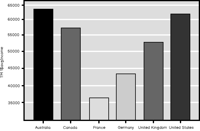
Finally, you can store the results of the dplyr functions in a normal data frame. The following code creates a new data frame and then shows the data graphically.
最后,您可以将dplyr函数的结果存储在普通数据框中。 以下代码创建一个新的数据框,然后以图形方式显示数据。
TM1 =
summarise(group_by(TM, Country), avgIncome = mean(Income))
barchart(TM1$avgIncome ~ TM1$Country)
The result is the following graph.
结果如下图。
先进的Python熊猫聚合 (Advanced Python Pandas Aggregations)
Time to switch to Python. Again, I need to start with importing the necessary libraries and reading the data.
是时候切换到Python了。 同样,我需要从导入必要的库并读取数据开始。
import numpy as np
import pandas as pd
import pyodbc
import matplotlib.pyplot as plt
con = pyodbc.connect('DSN=AWDW;UID=RUser;PWD=Pa$$w0rd')
query = """
SELECT g.EnglishCountryRegionName AS Country,
 c.EnglishEducation AS Education,
 c.YearlyIncome AS Income,
 c.NumberCarsOwned AS Cars
FROM dbo.DimCustomer AS c
 INNER JOIN dbo.DimGeography AS g
  ON c.GeographyKey = g.GeographyKey;"""
TM = pd.read_sql(query, con)
From the previous article, you probably remember the describe() function. The following code uses it to calculate the descriptive statistics for the Income variable over countries.
在上一篇文章中,您可能还记得describe()函数。 以下代码使用它来计算国家/地区收入变量的描述性统计数据。
TM.groupby('Country')['Income'].describe()
Here is an abbreviated result.
这是一个缩写结果。
Country
Australia       count      3591.000000
                mean      64338.624339
                std       31829.998608
                min       10000.000000
                25%       40000.000000
                50%       70000.000000
                75%       80000.000000
                max      170000.000000
Canada          count      1571.000000
                mean      57167.409293
                std       20251.523043
You can use the unstack() function to get a tabular result:
您可以使用unstack()函数获取表格结果:
TM.groupby('Country')['Income'].describe().unstack()
Here is the narrowed tabular result.
这是缩小的表格结果。
                 count          mean           std
Country
Australia       3591.0  64338.624339  31829.998608
Canada          1571.0  57167.409293  20251.523043
France          1810.0  35762.430939  27277.395389
Germany         1780.0  42943.820225  35493.583662
United Kingdom  1913.0  52169.367486  48431.988315
United States   7819.0  63616.830797  25706.482289
You can use the SQL aggregate() function to calculate multiple aggregates on multiple columns at the same time. The agg() is a synonym for the SQL aggregate(). Look at the following example.
您可以使用SQL Aggregate()函数同时计算多个列上的多个聚合。 agg()是SQL Aggregate()的同义词。 看下面的例子。
TM.groupby('Country').aggregate({'Income': 'std',
                                 'Cars':'mean'})
TM.groupby('Country').agg({'Income': ['max', 'mean'],
                           'Cars':['sum', 'count']})
The first call calculates a single SQL aggregate for two variables. The second call calculates two aggregates for two variables. Here is the result of the second call.
第一个调用为两个变量计算单个SQL聚合。 第二个调用为两个变量计算两个聚合。 这是第二次通话的结果。
                 Cars          Income
                  sum count       max          mean
Country
Australia        6863  3591  170000.0  64338.624339
Canada           2300  1571  170000.0  57167.409293
France           2259  1810  110000.0  35762.430939
Germany          2162  1780  130000.0  42943.820225
United Kingdom   2325  1913  170000.0  52169.367486
United States   11867  7819  170000.0  63616.830797
You might dislike the form of the previous result because the names of the columns are written in two different rows. You might want to flatten the names to a single word for a column. You can use the numpy ravel() function to latten the array of the column names and then concatenate them to a single name, like the following code shows.
您可能不喜欢上一个结果的形式,因为列的名称写在两个不同的行中。 您可能希望将名称拼合为一个列的单个单词。 您可以使用numpy ravel()函数对列名称的数组进行latten,然后将它们连接为单个名称,如以下代码所示。
# Renaming the columns
IncCars = TM.groupby('Country').aggregate(
    {'Income': ['max', 'mean'],
     'Cars':['sum', 'count']})
# IncCars
# Ravel function
# IncCars.columns
# IncCars.columns.ravel()
# Renaming
IncCars.columns = ["_".join(x) for x in IncCars.columns.ravel()]
# IncCars.columns
IncCars
You can also try to execute the commented code to get the understanding how the ravel() function works step by step. Anyway, here is the final result.
您也可以尝试执行注释的代码,以逐步了解ravel()函数的工作方式。 无论如何,这是最终结果。
                Cars_sum  Cars_count  Income_max   Income_mean
Country
Australia           6863        3591    170000.0  64338.624339
Canada              2300        1571    170000.0  57167.409293
France              2259        1810    110000.0  35762.430939
Germany             2162        1780    130000.0  42943.820225
United Kingdom      2325        1913    170000.0  52169.367486
United States      11867        7819    170000.0  63616.830797
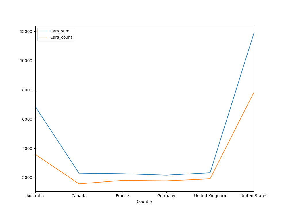
For a nice end, let me show you the results also graphically.
为了取得良好的效果,让我以图形方式向您显示结果。
IncCars[['Cars_sum','Cars_count']].plot()
plt.show()
And here is the graph.
这是图形。
结论 (Conclusion)
I will finish with aggregations in this data science series for now. However, I am not done with data preparation yet. You will learn about other problems and solutions in the forthcoming data science articles.
现在,我将结束本数据科学系列的汇总。 但是,我还没有完成数据准备。 您将在即将发表的数据科学文章中了解其他问题和解决方案。


 7537
7537

 被折叠的 条评论
为什么被折叠?
被折叠的 条评论
为什么被折叠?
 到【灌水乐园】发言


