


数据科学导论
Data science, machine learning, data mining, advanced analytics, or however you want to name it, is a hot topic these days. Many people would like to start some project in this area. However, very soon after the start you realize you have a huge problem: your data. Your data might come from your line of business applications, data warehouses, or even external sources. Typically, it is not prepared for applying advanced analytical algorithms on it straight out of the source. In addition, you have to understand your data thoroughly, otherwise you might feed the algorithms with inappropriate variables. Soon you learn the fact that is well known to seasoned data scientists: you spend around 70-80% of the time dedicated to a data science project on data preparation and understanding.
数据科学,机器学习,数据挖掘,高级分析,或者您想命名的,这些天都是热门话题。 许多人想在这个领域开始一些项目。 但是,在开始之后不久,您就意识到自己有一个巨大的问题:数据。 您的数据可能来自您的业务应用程序,数据仓库,甚至是外部来源。 通常,它不准备直接在源头上对其应用高级分析算法。 此外,您必须彻底理解数据,否则可能会给算法提供不合适的变量。 很快,您就会了解经验丰富的数据科学家所熟知的事实:您花费大约70-80%的时间专门用于数据科学项目,以进行数据准备和理解。
The whole data science project lifecycle is described with cross-industry standard process for data mining, by acronym CRISP-DM, described well in a Wikipedia article, which you can access by using this link. The following figure shows the process graphically.
整个数据科学项目的生命周期是通过跨行业的数据挖掘标准过程描述的,缩写为CRISP-DM,在Wikipedia文章中有很好的描述,您可以使用此链接进行访问。 下图以图形方式显示了该过程。
With this article, I am starting a series of articles on exactly these two issues, data understanding and data preparation. I will explain the problems and show the solutions in different programming languages, including T-SQL, R, and Python. I hope that you will find these articles valuable in your data science routines.
从本文开始,我将开始就这两个问题(数据理解和数据准备)这一系列文章。 我将用各种编程语言(包括T-SQL,R和Python)解释问题并显示解决方案。 我希望您会发现这些文章对您的数据科学例程很有用。
数据集,案例和变量 (Datasets, cases and variables)
As I mentioned, I will focus on the data understanding and preparation part only. But don’t forget that you need to have a god business problem understanding as well. By understanding your business problem, you can also understand the data much better. In data science, you analyze datasets that consist of cases, which are described by their variables. If you are working with SQL Server, then a dataset is represented by a table, where a case is a row and a variable is a column. In R and Python, you use the data frame objects to represent datasets to analyze. Data frames look like tables; however, they are matrices. This means that you can access the data positionally.
如前所述,我将只关注数据理解和准备部分。 但是请不要忘记,您还需要了解上帝的业务问题。 通过了解您的业务问题,您还可以更好地了解数据。 在数据科学中,您要分析由案例组成的数据集,这些案例由其变量描述。 如果使用的是SQL Server,则数据集由表表示,表中的大小写是一行,变量是列。 在R和Python中,您使用数据框对象表示要分析的数据集。 数据框看起来像表格。 但是,它们是矩阵。 这意味着您可以按位置访问数据。
The first issue you got is how to define a case. Sometimes it’s not so simple as you imagine. Let’s say that you need to analyze phone calls within a family and compare them to the calls outside a family. In this example, you might decide that your case is a single person, or a single family. Anyway, you prepare a dataset, where you gather together all information about your case.
您遇到的第一个问题是如何定义案例。 有时候,它并不像您想象的那么简单。 假设您需要分析家庭内部的电话,并将其与家庭外部的电话进行比较。 在此示例中,您可能会确定您的案件是一个人还是一个家庭。 无论如何,您都准备了一个数据集,在其中收集了有关案件的所有信息。
测量数据值的方法 (Ways to measure data values)
Your variables can measure values in different ways. Discrete variables can take a value only from a limited pool of values. For example, you might have information about the relationship status of your customers. You track only if the customer is married or is engaged in any other kind of relationship or single. The relationship status variable could then occupy two states only: “single” and “engaged”. Such a variable is categorical, or also called nominal variable.
您的变量可以用不同的方式测量值。 离散变量只能从有限的值池中获取值。 例如,您可能具有有关客户关系状态的信息。 仅在客户已婚或从事任何其他类型的关系或单身时跟踪您。 关系状态变量然后只能占据两个状态:“单个”和“已接合”。 这样的变量是分类变量,也称为名义变量。
Discrete variables can also have intrinsic order. You can rank the values; however, you cannot use any arithmetic on the values. Such variables are called ranks, or also ordinal variables. Education is a good example. There is an order between different possible values, or levels, of education.
离散变量也可以具有固有顺序。 您可以对值进行排名; 但是,您不能在值上使用任何算术。 这样的变量称为等级,也称为序数变量。 教育就是一个很好的例子。 教育的不同可能价值或水平之间是有序的。
There are also some specific discrete variables. If a variable can take only a single value, meaning the variable is actually a constant, then it is not useful for analysis, and you can simply drop it from the dataset. If a variable can take a value from a pool limited to two values only, like the relationship status I mentioned above, then this is a dichotomous variable. If you represent the stated with numbers 0 and 1 or false and true, using either integer or bit data type, then this is a binary variable.
还有一些特定的离散变量。 如果变量只能使用一个值,这意味着该变量实际上是一个常数,则它对分析没有用,您可以简单地将其从数据集中删除。 如果一个变量只能从一个池中将一个值限制为两个值,例如上面提到的关系状态,那么这就是一个二分变量。 如果使用整数或位数据类型用数字0和1或false和true表示声明,则这是一个二进制变量。
Variables can be also continuous, like numbers, or dates. Still, the pool of the possible values can be limited. Maybe you need to use the temperature of the air in your analysis. Of course, temperature is limited on the left side – it can’t go below absolute zero. Time intervals, like periods when somebody used a service, have a lower and an upper boundary. These variables are intervals. Arithmetic is many times somehow limited with such variables. Looking at the temperature example, subtraction of two temperatures might have sense, but addition not. You should check what arithmetic is allowed for every interval in your dataset.
变量也可以是连续的,例如数字或日期。 尽管如此,可能值的池仍可能受到限制。 也许您需要在分析中使用空气温度。 当然,温度在左侧是受限制的-它不能低于绝对零值。 时间间隔(例如有人使用服务的时间间隔)具有上下边界。 这些变量是间隔。 算术常常受到此类变量的限制。 从温度示例来看,将两个温度相减可能是有道理的,但相加则没有意义。 您应该检查数据集中每个时间间隔都允许使用哪种算法。
The least amount of problems usually come with true numeric variables, which are continuous and not limited on any side. They usually allow any kind of arithmetic operation on them.
真正的数字变量通常会带来最少的问题,它们是连续的,没有任何局限性。 它们通常允许对其进行任何算术运算。
Continuous variables might have a very specific distribution. Of course, you are familiar with the identity property or with sequences in SQL Server. Identity columns’ values are ever-growing. Such variables are monotonic. They might still be useful for your analysis. For example, a higher identity value might tell you that the case was introduced in the dataset later than the one with a lower value. Again, you should understand how your data is collected. You know that it is possible to insert identity values also manually, although this is not a very frequent case. However, if you cannot rely on the monotonic behavior of your identity columns, they might not be quite useful for further analysis.
连续变量可能具有非常特定的分布。 当然,您熟悉Identity属性或SQL Server中的序列。 标识列的值在不断增长。 这样的变量是单调的。 它们可能仍然对您的分析有用。 例如,较高的标识值可能会告诉您,该案例是在数据集中引入的,而不是较低的案例。 同样,您应该了解如何收集数据。 您知道也可以手动插入标识值,尽管这种情况不是很常见。 但是,如果您不能依赖标识列的单调性行为,则它们对于进一步分析可能没有太大用处。
离散变量概述 (Overview of discrete variables)
Overview of a variable actually means an overview of the variable’s distribution. You do this overview by using different kind of charts and descriptive statistics.
变量概述实际上是指变量分布的概述。 您可以使用其他类型的图表和描述性统计信息来进行此概述。
To see the distribution of discrete variables, you use frequency tables, or shortly frequencies. In a frequency table, you can show values, counts of those values, the percentage of the value count compared with the total count or the absolute percentage, the running total of the counts or the cumulative frequency, the running total of the percentages or the cumulative percent, and a bar char or a histogram of the counts.
要查看离散变量的分布,请使用频率表或简称频率。 在频率表中,您可以显示值,这些值的计数,与总计数或绝对百分比相比的值计数的百分比,计数或累积频率的累计,百分比或累计的累计累积百分比,以及条形图或计数的直方图。
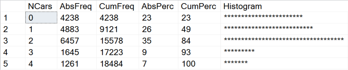
The following code shows how you can create a frequency table with T-SQL. I am using the AdventureWorksDW2016 demo database, the dbo.vTargetMail view as the dataset, and analyze the NumberCarsOwned variable. You can download the backup of this database from GitHub.
以下代码显示了如何使用T-SQL创建频率表。 我正在使用AdventureWorksDW2016演示数据库,将dbo.vTargetMail视图用作数据集,并分析NumberCarsOwned变量。 您可以从GitHub下载此数据库的备份。
USE AdventureWorksDW2016;
GO
WITH freqCTE AS
(
SELECT v.NumberCarsOwned,
 COUNT(v.NumberCarsOwned) AS AbsFreq,
 CAST(ROUND(100. * (COUNT(v.NumberCarsOwned)) /
       (SELECT COUNT(*) FROM vTargetMail), 0) AS INT) AS AbsPerc
FROM dbo.vTargetMail AS v
GROUP BY v.NumberCarsOwned
)
SELECT NumberCarsOwned AS NCars,
 AbsFreq,
 SUM(AbsFreq)
  OVER(ORDER BY NumberCarsOwned
       ROWS BETWEEN UNBOUNDED PRECEDING
	    AND CURRENT ROW) AS CumFreq,
 AbsPerc,
 SUM(AbsPerc)
  OVER(ORDER BY NumberCarsOwned
       ROWS BETWEEN UNBOUNDED PRECEDING
	    AND CURRENT ROW) AS CumPerc,
 CAST(REPLICATE('*',AbsPerc) AS VARCHAR(50)) AS Histogram
FROM freqCTE
ORDER BY NumberCarsOwned;
The following figure shows the results of the previous query.
下图显示了上一个查询的结果。
Of course, you can quickly do a similar overview with Python. If you are new to Python, I suggest you start with my introducing article about it, aimed at SQL Server specialists. You can execute this code in Visual Studio 2017. I explained the installation of SQL Server 2017 ML Services and Visual Studio 2017 for data science and analytical applications in the article I just mentioned. Here is the Python code.
当然,您可以使用Python快速进行类似的概述。 如果您不熟悉Python,建议您从针对SQL Server专家的介绍文章开始。 您可以在Visual Studio 2017中执行此代码。在我刚刚提到的文章中,我解释了SQL Server 2017 ML Services和Visual Studio 2017用于数据科学和分析应用程序的安装。 这是Python代码。
# Imports needed
import numpy as np
import pandas as pd
import pyodbc
import matplotlib.pyplot as plt

# Connecting and reading the data
con = pyodbc.connect('DSN=AWDW;UID=RUser;PWD=********')
query = """SELECT NumberCarsOwned
           FROM dbo.vTargetMail;"""
TM = pd.read_sql(query, con)

# Counts table and a bar chart
pd.crosstab(TM.NumberCarsOwned, columns = 'Count')
pd.crosstab(TM.NumberCarsOwned, columns = 'Count').plot(kind = 'bar')
plt.show()
This code produces the counts and also a nice graph, shown in the following figure.
这段代码会产生计数以及一个漂亮的图形,如下图所示。
Note that I used the ODBC Data Sources tool to create a system DSN called AWDW in advance. It points to my AdventureWorksDW2016 demo database. For the connection, I use the RUser SQL Server login I created specifically for Python and R. Of course, I created a database user in the AdventureWorksDW2016 database for this user and gave the user permission to read the data.
请注意,我使用ODBC数据源工具预先创建了一个称为AWDW的系统DSN。 它指向我的AdventureWorksDW2016演示数据库。 对于连接,我使用我专门为Python和R创建的RUser SQL Server登录名。当然,我在AdventureWorksDW2016数据库中为此用户创建了一个数据库用户,并授予该用户读取数据的权限。
Finally, let me show you and example in R. If you are new to R, I suggest you download the slides and the demos from my Introducing R session I delivered at the SQL Saturday #626 Budapest event. You will get also the link you need to download the RStudio IDE development tool in this presentation if you prefer this tool to Visual Studio. Anyway, here is the R code.
最后,让我向您展示R中的示例。如果您是R的新手,建议您从我在SQL Saturday#626 Budapest活动中介绍的R简介会话中下载幻灯片和演示。 如果您更喜欢Visual Studio,则还将获得此演示文稿中下载RStudio IDE开发工具所需的链接。 无论如何,这是R代码。
# Install and load RODBC library
install.packages("RODBC")
library(RODBC)

# Connecting and reading the data
con <- odbcConnect("AWDW", uid = "RUser", pwd = "********")
TM <- as.data.frame(sqlQuery(con,
  "SELECT NumberCarsOwned
   FROM dbo.vTargetMail;"),
  stringsAsFactors = TRUE)
close(con)

# Package descr
install.packages("descr")
library(descr)
freq(TM$NumberCarsOwned, col = 'light blue')
Note that in R, you typically need many additional packages. In this case, I used the descr package, which brings a lot of useful descriptive statistics functions. The freq() function I called returns a frequency table with counts and absolute percentages. In addition, it returns a graph, which you can see in the following figure.
请注意,在R中,您通常需要许多其他软件包。 在这种情况下,我使用了descr包,它带来了许多有用的描述性统计功能。 我调用的freq()函数返回带有计数和绝对百分比的频率表。 此外,它还返回一个图形,您可以在下图中看到它。
结论 (Conclusion)
This article is just a small teaser, a brief introduction of the big amount of work with data overview and preparation for data science projects. In my following articles, I intend to add quite a few more articles on this topic, with more advanced problems explained and resolved, and with more statistical procedures used for in-depth data understanding.
本文只是一个小预告片,简要介绍了数据概述和为数据科学项目做准备的大量工作。 在接下来的文章中,我打算添加更多关于该主题的文章,解释和解决更高级的问题,并使用更多的统计程序来深入理解数据。
目录 (Table of contents)
资料下载 (Downloads)
参考资料 (References)
- Introduction to Python Python简介
- Introduction to R R简介
- Python Pandas.DataFrame Python Pandas.DataFrame
- R Tutorial: Data Frame R教程:数据框
- The descr package documentation descr软件包文档
- SELECT – OVER Clause (Transact-SQL) SELECT – OVER子句(Transact-SQL)
翻译自: https://www.sqlshack.com/introduction-to-data-science-data-understanding-and-preparation/
数据科学导论


 1051
1051

 被折叠的 条评论
为什么被折叠?
被折叠的 条评论
为什么被折叠?
 到【灌水乐园】发言


