神经网络简介：第1部分

We use our most advanced technologies as metaphors for the brain: The industrial revolution inspired descriptions of the brain as mechanical. The telephone inspired descriptions of the brain as a telephone switchboard. The computer inspired descriptions of the brain as a computer. Recently, we have reached a point where our most advanced technologies – such as AI (e.g., Alpha Go), and our current understanding of the brain inform each other in an awesome synergy. Neural networks exemplify this synergy. Neural networks offer a relatively advanced description of the brain and are the software underlying some of our most advanced technology. As our understanding of the brain increases, neural networks become more sophisticated. As our understanding of neural networks increases, our understanding of the brain becomes more sophisticated.

我们使用最先进的技术作为大脑的隐喻：工业革命激发了人们对机械的描述。 电话激发了人们对大脑作为电话总机的描述。 计算机激发了将大脑描述为计算机的描述。 最近，我们达到了最先进的技术-如AI（例如Alpha Go ）和我们目前对大脑的了解，从而达到了令人敬畏的协同作用。 神经网络例证了这种协同作用。 神经网络提供了相对高级的大脑描述，并且是我们某些最先进技术的基础软件。 随着我们对大脑的了解增加，神经网络变得越来越复杂。 随着我们对神经网络的了解增加，对大脑的了解也越来越复杂。

With the recent success of neural networks, I thought it would be useful to write a few posts describing the basics of neural networks.

随着神经网络的最近成功，我认为写一些描述神经网络基础知识的文章会很有用。

First, what are neural networks – neural networks are a family of machine learning algorithms that can learn data’s underlying structure. Neural networks are composed of many neurons that perform simple computations. By performing many simple computations, neural networks can answer even the most complicated problems.

首先，什么是神经网络 –神经网络是一系列机器学习算法，可以学习数据的基础结构。 神经网络由执行简单计算的许多神经元组成。 通过执行许多简单的计算，神经网络甚至可以回答最复杂的问题。

Lets get started.

让我们开始吧。

As usual, I will post this code as a jupyter notebook on my github.

和往常一样，我会将这段代码作为jupyter笔记本发布在github上 。

1 1 2 2 3 3 4 4

When talking about neural networks, it’s nice to visualize the network with a figure. For drawing the neural networks, I forked a repository from miloharper and made some changes so that this repository could be imported into python and so that I could label the network. Here is my forked repository.

在谈论神经网络时，最好用数字形象化网络。 为了绘制神经网络，我从miloharper派生了一个存储库，并进行了一些更改，以便可以将该存储库导入python并为网络添加标签。 这是我的分叉存储库。

1 1 2 2 3 3 4 4 5 5 6 6 7 7

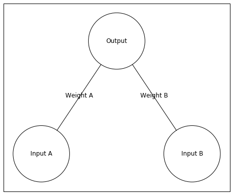
Above is our neural network. It has two input neurons and a single output neuron. In this example, I’ll give the network an input of [0 1]. This means Input A will receive an input value of 0 and Input B will have an input value of 1.

以上是我们的神经网络。 它具有两个输入神经元和一个输出神经元。 在此示例中，我将为网络输入[0 1]。 这意味着输入A的输入值为0，输入B的输入值为1。

The input is the input unit’s activity. This activity is sent to the Output unit, but the activity changes when traveling to the Output unit. The weights between the input and output units change the activity. A large positive weight between the input and output units causes the input unit to send a large positive (excitatory) signal. A large negative weight between the input and output units causes the input unit to send a large negative (inhibitory) signal. A weight near zero means the input unit does not influence the output unit.

输入是输入单元的活动。 该活动已发送到输出单元，但是在移动到输出单元时该活动会更改。 输入和输出单位之间的权重会更改活动。 输入单元和输出单元之间较大的正重量会导致输入单元发送较大的正（激励）信号。 输入单元和输出单元之间较大的负重量会导致输入单元发送较大的负（抑制）信号。 权重接近零表示输入单元不影响输出单元。

In order to know the Output unit’s activity, we need to know its input. I will refer to the output unit’s input as . Here is how we can calculate

为了知道输出单元的活动，我们需要知道其输入。 我将输出单元的输入称为。 这是我们如何计算

a more general way of writing this is

更一般的写法是

Let’s pretend the inputs are [0 1] and the Weights are [0.25 0.5]. Here is the input to the output neuron –

假设输入为[0 1]，权重为[0.25 0.5]。 这是输出神经元的输入-

Thus, the input to the output neuron is 0.5. A quick way of programming this is through the function numpy.dot which finds the dot product of two vectors (or matrices). This might sound a little scary, but in this case its just multiplying the items by each other and then summing everything up – like we did above.

因此，输出神经元的输入为0.5。 一种快速的编程方式是通过函数numpy.dot，该函数查找两个向量（或矩阵）的点积 。 这听起来可能有些吓人，但是在这种情况下，它只是将项目彼此相乘​​，然后将所有内容相加-就像我们上面所做的那样。

1 1 2 2 3 3 4 4 5 5

0.5
0.5
 

All this is good, but we haven’t actually calculated the output unit’s activity we have only calculated its input. What makes neural networks able to solve complex problems is they include a non-linearity when translating the input into activity. In this case we will translate the input into activity by putting the input through a logistic function.

所有这些都很好，但是我们实际上还没有计算出输出单元的活动，仅计算了其输入。 使神经网络能够解决复杂问题的原因是，当将输入转换为活动时，它们包括非线性。 在这种情况下，我们将通过逻辑函数将输入转化为活动。

def logistic(x): #each neuron has a logistic activation function return 1.0/(1+np.exp(-x)) def logistic ( x ): #each neuron has a logistic activation function return 1.0 / ( 1 + np . exp ( - x ))

Lets take a look at a logistic function.

让我们看一下物流功能。

x = np.arange(-5,5,0.1) #create vector of numbers between -5 and 5 plt.plot(x,logistic(x)) plt.ylabel('Activation') plt.xlabel('Input'); x = np . arange ( - 5 , 5 , 0.1 ) #create vector of numbers between -5 and 5 plt . plot ( x , logistic ( x )) plt . ylabel ( 'Activation' ) plt . xlabel ( 'Input' );

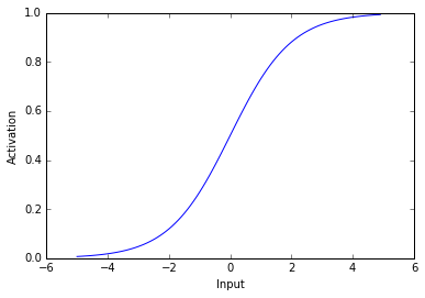
As you can see above, the logistic used here transforms negative values into values near 0 and positive values into values near 1. Thus, when a unit receives a negative input it has activity near zero and when a unit receives a postitive input it has activity near 1. The most important aspect of this activation function is that its non-linear – it’s not a straight line.

如上所示，这里使用的逻辑将负值转换为接近0的值，将正值转换为接近1的值。因此，当一个单元接收到负输入时，它的活动接近于零，而当一个单元接收到正输入时，它的活动就到了。接近1.此激活函数的最重要方面是非线性的-它不是直线。

Now lets see the activity of our output neuron. Remember, the net input is 0.5

现在，让我们看看输出神经元的活动。 记住，净输入为0.5

Output_neuron = logistic(net_Output) print Output_neuron plt.plot(x,logistic(x)); plt.ylabel('Activation') plt.xlabel('Input') plt.plot(net_Output,Output_neuron,'ro'); Output_neuron = logistic ( net_Output ) print Output_neuron plt . plot ( x , logistic ( x )); plt . ylabel ( 'Activation' ) plt . xlabel ( 'Input' ) plt . plot ( net_Output , Output_neuron , 'ro' );

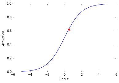
The activity of our output neuron is depicted as the red dot.

我们的输出神经元的活动表示为红点。

So far I’ve described how to find a unit’s activity, but I haven’t described how to find the weights of connections between units. In the example above, I chose the weights to be 0.25 and 0.5, but I can’t arbitrarily decide weights unless I already know the solution to the problem. If I want the network to find a solution for me, I need the network to find the weights itself.

到目前为止，我已经描述了如何查找单元的活动，但是还没有描述如何查找单元之间的连接权重。 在上面的示例中，我将权重选择为0.25和0.5，但是除非我已经知道问题的解决方案，否则我将无法任意决定权重。 如果我想让网络找到适合我的解决方案，则需要网络来寻找权重本身。

In order to find the weights of connections between neurons, I will use an algorithm called backpropogation. In backpropogation, we have the neural network guess the answer to a problem and adjust the weights so that this guess gets closer and closer to the correct answer. Backpropogation is the method by which we reduce the distance between guesses and the correct answer. After many iterations of guesses by the neural network and weight adjustments through backpropogation, the network can learn an answer to a problem.

为了找到神经元之间连接的权重，我将使用一种称为反向传播的算法。 在反向传播中，我们使神经网络猜测问题的答案并调整权重，以使该猜测越来越接近正确的答案。 反向传播是我们减少猜测和正确答案之间距离的方法。 在经过神经网络的猜测多次迭代以及通过反向传播进行权重调整之后，网络可以学习问题的答案。

Lets say we want our neural network to give an answer of 0 when the left input unit is active and an answer of 1 when the right unit is active. In this case the inputs I will use are [1,0] and [0,1]. The corresponding correct answers will be [0] and [1].

假设我们希望我们的神经网络在左输入单元激活时给出0的答案，而在右输入单元激活时给出1的答案。 在这种情况下，我将使用的输入为[1,0]和[0,1]。 相应的正确答案将是[0]和[1]。

Lets see how close our network is to the correct answer. I am using the weights from above ([0.25, 0.5]).

让我们看看我们的网络离正确答案有多近。 我正在使用上面的权重（[0.25，0.5]）。

1 1 2 2 3 3 4 4 5 5 6 6 7 7 8 8 9 9 10 10 11 11

[0.56217650088579807, 0.62245933120185459]
[0.56217650088579807, 0.62245933120185459]
 

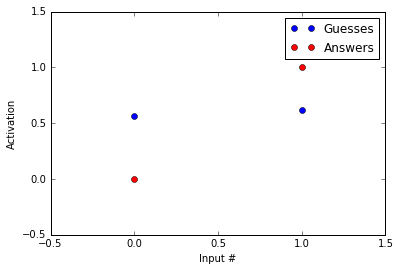
The guesses are in blue and the answers are in red. As you can tell, the guesses and the answers look almost nothing alike. Our network likes to guess around 0.6 while the correct answer is 0 in the first example and 1 in the second.

猜测为蓝色，答案为红色。 如您所知，猜测和答案几乎没有相似之处。 我们的网络喜欢猜测0.6，而正确的答案在第一个示例中为0，在第二个示例中为1。

Lets look at how backpropogation reduces the distance between our guesses and the correct answers.

让我们看一下反向传播如何减少我们的猜测与正确答案之间的距离。

First, we want to know how the amount of error changes with an adjustment to a given weight. We can write this as

首先，我们想知道在调整给定重量后误差量如何变化。 我们可以这样写

This change in error with changes in the weights has a number of different sub components.

权重变化带来的误差变化具有许多不同的子组件。

• Changes in error with changes in the output unit’s activity:
• Changes in the output unit’s activity with changes in this unit’s input:
• Changes in the output unit’s input with changes in the weight:

• 错误随输出单元活动的变化而变化：
• 输出单元的活动随该单元输入的改变而变化：
• 输出单元的输入随重量的变化而变化：

Through the chain rule we know

通过链式规则，我们知道

This might look scary, but with a little thought it should make sense: (starting with the final term and moving left) When we change the weight of a connection to a unit, we change the input to that unit. When we change the input to a unit, we change its activity (written Output above). When we change a units activity, we change the amount of error.

这可能看起来很吓人，但经过一点思考，它应该是有道理的：（从最后一项开始，然后向左移动）当我们更改某个单元的连接权重时，我们将更改该单元的输入。 当我们将输入更改为单位时，我们将更改其活动（上面编写了Output）。 当我们更改单位活动时，我们将更改错误量。

Let’s break this down using our example. During this portion, I am going to gloss over some details about how exactly to derive the partial derivatives. Wikipedia has a more complete derivation.

让我们用我们的例子来分解一下。 在这一部分中，我将介绍有关如何精确导出偏导数的一些细节。 维基百科具有更完整的派生形式 。

In the first example, the input is [1,0] and the correct answer is [0]. Our network’s guess in this example was about 0.56.

在第一个示例中，输入为[1,0]，正确答案为[0]。 在此示例中，我们的网络猜测约为0.56。

– Please note that this is specific to our example with a logistic activation function

–请注意，这特定于我们的具有逻辑激活功能的示例

to summarize (the numbers used here are approximate)

总结（此处使用的数字为近似值）

This is the direction we want to move in, but taking large steps in this direction can prevent us from finding the optimal weights. For this reason, we reduce our step size. We will reduce our step size with a parameter called the learning rate (). is bound between 0 and 1.

这是我们要前进的方向，但是朝这个方向大步前进可能会阻止我们找到最佳权重。 因此，我们减小步长。 我们将使用称为学习率（）的参数来减小步长。 介于0和1之间。

Here is how we can write our change in weights

这是我们写权重变化的方法

This is known as the delta rule.

这称为增量规则 。

We will set to be 0.5. Here is how we will calculate the new .

我们将设为0.5。 这是我们将如何计算新的。

Thus, is shrinking which will move the output towards 0. Below I write the code to implement our backpropogation.

因此，正在缩小，这会将输出移向0。在下面，我编写代码来实现反向传播。

alpha = 0.5 def delta_Output(target,Output): return -(target-Output)*Output*(1-Output) #find the amount of error and derivative of activation function def update_weights(alpha,delta,unit_input): return alpha*np.outer(delta,unit_input) #multiply delta output by all the inputs and then multiply these by the learning rate alpha = 0.5 def delta_Output ( target , Output ): return - ( target - Output ) * Output * ( 1 - Output ) #find the amount of error and derivative of activation function def update_weights ( alpha , delta , unit_input ): return alpha * np . outer ( delta , unit_input ) #multiply delta output by all the inputs and then multiply these by the learning rate

Above I use the outer product of our delta function and the input in order to spread the weight changes to all lines connecting to the output unit.

上面我使用了增量函数和输入的外部乘积 ，以便将权重变化分布到连接到输出单元的所有线上。

Okay, hopefully you made it through that. I promise thats as bad as it gets. Now that we’ve gotten through the nasty stuff, lets use backpropogation to find an answer to our problem.

好的，希望您能做到这一点。 我保证那会变得糟透了。 现在我们已经解决了令人讨厌的问题，让我们使用反向传播来找到问题的答案。

def network_guess(Input,Weights): return logistic(np.dot(Input,Weights.T)) #input by weights then through a logistic def back_prop(Input,Output,target,Weights): delta = delta_Output(target,Output) #find delta portion delta_weight = update_weights(alpha,delta,Input) #find amount to update weights Weights = np.atleast_2d(Weights) #convert weights to array Weights += -delta_weight #update weights return Weights from random import choice, seed seed(1) #seed random number generator so that these results can be replicated Weights = np.array([0.25, 0.5]) Error = [] while True: Trial_Type = choice([0,1]) #generate random number to choose between the two inputs Input = np.atleast_2d(Inputs[Trial_Type]) #choose input and convert to array Answer = Answers[Trial_Type] #get the correct answer Output = network_guess(Input,Weights) #compute the networks guess Weights = back_prop(Input,Output,Answer,Weights) #change the weights based on the error Error.append(abs(Output-Answer)) #record error if len(Error) > 6 and np.mean(Error[-5:]) < 0.05: break #tell the code to stop iterating when mean error is < 0.05 in the last 5 guesses def network_guess ( Input , Weights ): return logistic ( np . dot ( Input , Weights . T )) #input by weights then through a logistic def back_prop ( Input , Output , target , Weights ): delta = delta_Output ( target , Output ) #find delta portion delta_weight = update_weights ( alpha , delta , Input ) #find amount to update weights Weights = np . atleast_2d ( Weights ) #convert weights to array Weights += - delta_weight #update weights return Weights from random import choice , seed seed ( 1 ) #seed random number generator so that these results can be replicated Weights = np . array ([ 0.25 , 0.5 ]) Error = [] while True : Trial_Type = choice ([ 0 , 1 ]) #generate random number to choose between the two inputs Input = np . atleast_2d ( Inputs [ Trial_Type ]) #choose input and convert to array Answer = Answers [ Trial_Type ] #get the correct answer Output = network_guess ( Input , Weights ) #compute the networks guess Weights = back_prop ( Input , Output , Answer , Weights ) #change the weights based on the error Error . append ( abs ( Output - Answer )) #record error if len ( Error ) > 6 and np . mean ( Error [ - 5 :]) < 0.05 : break #tell the code to stop iterating when mean error is < 0.05 in the last 5 guesses

It seems our code has found an answer, so lets see how the amount of error changed as the code progressed.

看来我们的代码找到了答案，所以让我们看看随着代码的进展，错误量如何变化。

Error_vec = np.array(Error)[:,0] plt.plot(Error_vec) plt.ylabel('Error') plt.xlabel('Iteration #'); Error_vec = np . array ( Error )[:, 0 ] plt . plot ( Error_vec ) plt . ylabel ( 'Error' ) plt . xlabel ( 'Iteration #' );

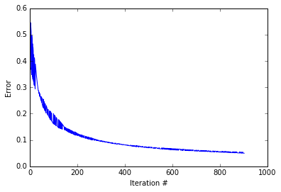
It looks like the while loop excecuted about 1000 iterations before converging. As you can see the error decreases. Quickly at first then slowly as the weights zone in on the correct answer. lets see how our guesses compare to the correct answers.

看起来，while循环在收敛之前执行了约1000次迭代。 如您所见，错误减少了。 首先快速然后缓慢，因为权重区域位于正确的答案上。 让我们看看我们的猜测如何与正确答案进行比较。

Inputs = [[1,0],[0,1]] Answers = [0,1,] Guesses = [logistic(np.dot(x,Weights.T)) for x in Inputs] #loop through inputs and find logistic(sum(input*weights)) plt.plot(Guesses,'bo') plt.plot(Answers,'ro') plt.axis([-0.5,1.5,-0.5,1.5]) plt.ylabel('Activation') plt.xlabel('Input #') plt.legend(['Guesses','Answers']); print Guesses Inputs = [[ 1 , 0 ],[ 0 , 1 ]] Answers = [ 0 , 1 ,] Guesses = [ logistic ( np . dot ( x , Weights . T )) for x in Inputs ] #loop through inputs and find logistic(sum(input*weights)) plt . plot ( Guesses , 'bo' ) plt . plot ( Answers , 'ro' ) plt . axis ([ - 0.5 , 1.5 , - 0.5 , 1.5 ]) plt . ylabel ( 'Activation' ) plt . xlabel ( 'Input #' ) plt . legend ([ 'Guesses' , 'Answers' ]); print Guesses

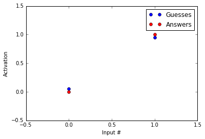
Not bad! Our guesses are much closer to the correct answers than before we started running the backpropogation procedure! Now, you might say, “HEY! But you haven’t reached the correct answers.” That’s true, but note that acheiving the values of 0 and 1 with a logistic function are only possible at – and , respectively. Because of this, we treat 0.05 as 0 and 0.95 as 1.

不错！ 与开始运行反向传播过程之前相比，我们的猜测更接近正确答案！ 现在，您可能会说：“嗨！ 但是您还没有得到正确的答案。” 没错，但是请注意，仅可以在–和处使用逻辑函数实现0和1的值。 因此，我们将0.05视为0，将0.95视为1。

翻译自: https://www.pybloggers.com/2016/04/an-introduction-to-neural-networks-part-1/