提升您的Hibernate引擎

1引言

Hibernate是提供数据持久性和查询服务的最流行的对象关系映射（ORM）引擎之一。

将Hibernate引入您的项目并使其正常工作很简单。 但是，要使其表现良好，确实需要时间和大量的经验。

本文使用在Hibernate 3.3.1和Oracle 9i的能源项目中找到的示例，介绍了许多Hibernate调整技术。 它还提供了一些数据库知识，您需要这些知识才能真正掌握一些Hibernate调整技术。

我们假设对Hibernate有基本的了解。 如果Hibernate参考文档（以下简称HRD）或其他优化文章中充分介绍了一种调优方法，我们将只提供对该文档的参考，并从不同的角度进行简要说明。 我们专注于有效的调优方法，但文献记载不充分。

2Hibernate性能调优

调整是一个反复不断的过程，涉及软件开发生命周期（SDLC）的所有阶段。 在使用Hibernate进行持久化的典型Java EE应用程序中，调优涉及以下领域：

• 调整业务规则
• 调音设计
• 调整Hibernate
• 调优Java GC
• 调整应用程序容器
• 调整基础系统，包括数据库和OS。

在没有精心计划的方法的情况下对所有这些参数进行调整非常耗时，并且可能效果不佳。 好的调整方法的重要部分是确定调整区域的优先级。 可以用帕累托原理（又名“ 80/20规则”）解释，该原则说大约80％的应用程序性能改进来自所有性能问题中排在前20％的问题^[5] 。

与基于磁盘和网络的访问相比，基于内存和CPU的访问可以提供更低的延迟和更高的吞吐量。 鉴于这种基于Hibernate的IO调优以及基础系统的IO部分，应优先于基于GC和基于CPU的内存调优以及基础系统的CPU和内存部分。

例子1

我们调整了HQL查询，以选择大约30秒到不到1秒的电力交易。 如果我们在垃圾收集器上进行工作，则改进的幅度可能会小得多，最多可能只有几毫秒或几秒钟，而与HQL的改进相比，这对于交易员来说是不明显的。

好的调整方法的另一个重要部分是决定何时进行优化^[4] 。

积极的调优倡导者从一开始即在业务规则和设计阶段就开始进行调优，并在整个SDLC上进行调优，因​​为他们认为更改业务规则和以后重新设计通常非常昂贵。

积极的倡导者在SDLC的结尾提倡调优，因为他们抱怨提早调优通常会使设计和编码变得复杂。 他们经常引用Donald Knuth ^[6]流行的短语“ 过早的优化是万恶之源 ”。

需要权衡以平衡调整和编码。 作者的经验表明，适当的早期调整会导致更谨慎的设计和更仔细的编码。 许多项目因应用程序调整而失败，因为上面的“过早优化”一词是在上下文之外引用的，因此调整要么被推到了项目的最后，要么资源太少。

但是，进行大量的早期调整并不总是可行的，因为如果不先对其进行概要分析就无法确切知道应用程序的瓶颈在哪里，那么在此之上应用程序通常仍在不断发展。

对我们的多线程企业应用程序进行性能分析还表明，大多数应用程序平均只有20-50％的CPU使用率。 其余的CPU只是等待数据库和网络相关IO的开销。

根据以上分析，我们得出的结论是，根据帕累托原理调整Hibernate以及业务规则和设计属于20％，因此，它们应该具有最高优先级。

一种实用的方法如下：

1. 确定主要瓶颈，可以预测到的大多数瓶颈以及业务规则和设计（数量取决于您的调整目标；但是三到五个是一个好的开始）。
2. 修改您的应用程序以消除它们。
3. 测试您的应用程序，然后再次从第1步重复进行，直到达到调整目标。

关于性能调优策略的更多一般性建议可以在Jack Shirazi的书“ Java Performance Tuning”中找到^[7] 。

在以下各节中，我们以调优影响的大致顺序说明特定的调优技术（也就是说，首先列出的那些通常具有最大的影响）。

3监视和分析

如果没有对Hibernate应用程序进行足够的监视和分析，您将不会知道性能瓶颈在哪里以及需要调整哪些部分。

3.1.1监视SQL生成

尽管使用Hibernate的主要目的是使您免于直接处理SQL，但您必须知道SQL Hibernate生成了什么以调整应用程序。 乔尔·斯普洛斯基（Joel Splosky）在他的文章《泄漏抽象法则》中很好地阐述了这个问题。

您可以在log4j中将org.hibernate.SQL包的日志级别打开为DEBUG，以查看生成的所有SQL。 您可能还需要将其他软件包的日志级别设置为DEBUG，甚至TRACE，以查明一些性能问题。

3.1.2检查Hibernate统计信息

如果启用hibernate.generate.statistics ，则Hibernate将公开有关实体，集合，会话，二级缓存，查询和会话工厂的指标，这些指标对于通过SessionFactory.getStatistics（）进行调整非常有用。 为了使生活更轻松，Hibernate还可以使用MBean“ org.hibernate.jmx.StatisticsService ”通过JMX公开指标。 您可以从该网站找到配置示例。

3.1.3分析

一个好的性能分析工具不仅有益于您的Hibernate调优，还有益于应用程序的其他部分。 但是，大多数商业工具（例如JProbe ^[10]）非常昂贵。 幸运的是，Sun / Oracle的JDK 1.6包含一个称为“ Java VisualVM”的分析接口^[11] 。 与商业对手相比，这是相当基本的。 但是，它确实提供了许多调试和调整信息。

4种调音技巧

4.1调整业务规则和设计

尽管调优业务规则和设计本身并不属于Hibernate调优，但调优的决定对下游的Hibernate调优有很大影响。 因此，我们重点介绍了与Hibernate调整有关的一些要点。

通过业务需求收集和调整，您应该知道：

• 数据检索特性包括参考数据，只读数据，读取组，读取大小，搜索条件以及数据分组和聚合。
• 数据修改特征包括数据更改，更改组，更改大小，错误的修改许可，数据库（所有更改是在一个数据库中还是在多个数据库中？），更改频率和并发性以及更改响应和吞吐量要求。
• 数据关系，例如关联，概括，实现和依赖性。

根据业务需求，您将得出最佳设计，在此设计中您可以确定应用程序类型（在线事务处理（OLTP）或数据仓库，或接近两者）和层结构（单独的持久性和服务层或组合），进行创建域对象通常作为POJO并决定数据聚合位置（数据库中的聚合利用了强大的数据库功能并节省了网络带宽；但是，除了COUNT，SUM，AVG，MIN和MAX等标准聚合外，它通常不可移植。在应用程序服务器中，您可以应用更复杂的业务逻辑；但是您需要先将详细的数据加载到应用程序层。

例子2

分析师需要从大型DB表中查看ISO（独立系统运营商）交易的汇总列表。 最初，他们想显示大多数表列。 该应用程序花费了30分钟的时间，因为它最多向前端UI加载了100万行，即使数据库在1分钟之内做出了响应。 重新分析后，分析人员除去了14根色谱柱。 由于取消了许多可选的高基数列，因此其余列的聚合分组返回的数据比以前少得多，并且在大多数情况下，数据加载时间被缩短为可以接受的。

例子3

电力每小时交易者经常修改24小时的定额小时，其中包括2个属性：小时电量和价格（“定额”是指每个小时可以有自己的量和价格；如果所有24小时都具有相同的量和价格，我们称它们为“标准” ）。 最初，我们使用Hibernate的select-before-update功能，这意味着更新24行需要24个选择。 因为我们只有2个属性，并且没有业务规则禁止在数量或价格不变的情况下进行错误更新，所以我们关闭了“ 更新前选择”功能，并避免了24个选择。

4.2调整继承映射

尽管继承映射是域对象的一部分，但由于其重要性，我们将其分开对待。 HRD ^[9]中的 第9章“继承映射”已经介绍了很多，因此我们将重点介绍SQL生成和每种策略的调整建议。

这是HRD中示例的类图：

[该图包括“ CreditCardType”，但所有后续SQL均引用“ cc_type”]

4.2.1每个类层次结构的表

只需一张桌子。 多态查询会生成SQL，例如：

select id, payment_type, amount, currency, rtn, credit_card_typefrom payment

从具体子类（如CashPayment）上的查询生成SQL看起来像：

select id, amount, currencyfrom payment where payment_type=’CASH’ 

优点包括单个表，简单的查询以及与其他表的轻松关联。 同样，第二个查询不需要在其他子类中包含属性。 所有这些功能使性能调整比其他策略容易得多。 该方法通常非常适合数据仓库系统，因为所有数据都在一个表中，而无需表联接。

主要缺点是在整个类层次结构中有一个包含所有属性的大表。 如果类层次结构具有许多特定于子类的属性，则数据库中将有太多的空列值，这将使当前基于行的数据库难以进行SQL调整（使用基于列的DBMS的数据仓库系统可以更好地解决此问题）。 因为除非对其进行分区，否则唯一的表可能是热点，因此OLTP系统通常无法很好地使用它。

4.2.2每个子类的表

需要四个表。 多态查询生成SQL

select id, payment_type, amount, currency, rtn, credit_card type,
        case when c.payment_id is not null then 1
             when ck.payment_id is not null then 2
             when cc.payment_id is not null then 3
             when p.id is not null then 0 end as clazz
from payment p left join cash_payment c on p.id=c.payment_id left join
   cheque_payment ck on p.id=ck.payment_id left  join 
   credit_payment cc on p.id=cc.payment_id; 

从具体子类（如CashPayment）上的查询生成SQL看起来像：

select id, payment_type, amount, currency
from payment p left join cash_payment c on p.id=c.payment_id; 

优点包括紧凑表（没有不必要的可为空的列），跨三个子类表的数据分区以及使用顶级超类表轻松与其他表关联的功能。 紧凑表可以优化基于行的数据库的存储块，从而使SQL性能更好。 数据分区增加了数据更改的并发性（除了超类之外没有热点），因此OLTP系统通常会处理它

同样，第二个查询不需要在其他子类中包含属性。

缺点包括所有策略中最多的表和外部联接以及稍微复杂SQL（请查看Hibernate动态标识符的CASE子句长）。 由于数据库在调整表联接上花费的时间比单个表花费更多的时间，因此数据仓库通常无法很好地与之配合使用。

因为您不能使用超类和子类中的列来创建复合数据库索引，所以如果您需要查询此类列，则会降低性能。 同样，子类上的任何数据更改都涉及两个表：超类表和子类表。

4.2.3每个具体类别的表格

涉及三个或更多表。 多态查询生成如下SQL：

select p.id, p.amount, p.currency, p.rtn, p. credit_card_type, p.clazz
from ( select id, amount, currency, null as rtn, null as credit_card type,
             1 as clazz from cash_payment union all
      select id, amount, null as currency, rtn, null as credit_card type,
             2 as clazz from cheque_payment union all
      select id, amount, null as currency, null as rtn,credit_card type,
             3 as clazz from credit_payment) p; 

从具体子类（如CashPayment）上的查询生成SQL看起来像：

select id, payment_type, amount, currency from cash_payment; 

优点类似于上面的“每个子类的表”策略。 因为超类通常是抽象的，并且恰好需要三个表[开始时说需要三个或三个以上]，所以子类上的任何数据更改仅涉及一个表，因此运行速度更快。

缺点包括复杂SQL（from子句中的子查询，并并集全部）。 但是，大多数数据库都可以很好地调整此类SQL。

如果一个类想与超级支付类相关联，则数据库不能使用参照完整性来实施它。 您必须使用触发器来执行此操作。 这会使数据库性能受到影响。

4.2.4使用隐式多态性的每个具体类的表

只需要三个表。 Payment上的多态查询生成三个单独SQL语句，每个语句都在一个子类上。 Hibernate引擎使用Java反射来找出Payment的所有三个子类。

对具体子类的查询只会为该子类生成SQL。 这些SQL语句非常简单，因此在此处被忽略。

优点与上一节类似：紧凑表，跨三个具体子类表的数据分区以及子类上的任何数据更改仅涉及一个表。

缺点包括三个单独SQL语句，而不是一个联合SQL语句，这会导致更多的网络IO。 Java反射也需要时间。 想象一下，如果您有大量的域对象并且隐式地从顶级Object类中进行选择，将花费多长时间。

为您的映射策略做出合理的选择并不容易； 它要求您仔细调整业务需求并根据您的特定数据方案做出合理的设计决策。

以下是我们的建议：

• 设计细粒度的类层次结构和粗粒度的数据库表。 拥有细粒度的数据库表意味着更多的表联接以及相应的更复杂的查询。
• 如果不需要多态查询，请不要使用它们。 如上所示，对具体类的查询仅选择所需的数据，而没有不必要的表联接或联合。
• “按类分类的表”适用于数据仓库系统（基于列的数据库）以及具有低并发性且共享大多数列的OLTP系统。
• “每个子类的表”适用于具有高并发性，简单查询和少量共享列的OLTP系统。 如果要使用数据库参照完整性来强制关联，这也是一个明智的选择。
• “每个具体类的表”适用于具有高并发性，复杂查询和少量共享列的OLTP系统。 当然，您必须牺牲超类和其他类之间的关联。
• 诸如“每个类的表”中嵌入的“每个子类的表”之类的混合策略，使您可以利用不同的策略。 如果您必须随着项目的发展做出React性的重新设计映射策略，那么您可能还会诉诸于此
• 不建议使用“使用隐式多态性的每个具体类的表”，因为它的配置冗长，使用“ any”元素的复杂关联语法以及潜在的危险隐式查询。

例子4

这是交易捕获应用程序的域类图的一部分：

最初，该项目只有GasDeal和少量的用户群。 它使用“每个类层次结构的表”。

后来，当出现更多业务需求时，添加了OilDeal和ElectricityDeal。 没有更改映射策略。 但是ElectricityDeal有太多自己的属性。 因此，许多特定于电力的可空列已添加到“交易”表中。 由于用户群也不断增长，因此数据更改变得越来越慢。

对于重新设计，我们针对燃气/石油和电力的特定属性采用了两个单独的表。 新的映射是“按类分类的表”和“按子类分类的表”的混合体。 我们还重新设计了查询，以允许在具体的交易子类上进行选择，以消除不必要的表列和联接。

4.3调整域对象

基于第4.1节中业务规则和设计的调整，您为POJO表示的域对象提供了一个类图。 我们的建议是：

4.3.1调整POJO

• 从只读数据中分离出诸如引用之类的只读数据，以及以读写为主的数据。
  只读数据的第二级缓存是最有效的，其次是对大多数读数据进行非严格读写。 您还可以将不可变的只读POJO标记为调整提示。 如果服务层方法仅处理只读数据，则可以将其事务标记为只读，这是优化Hibernate和基础JDBC驱动程序的提示。
• 细粒度的POJO和粗粒度的数据库表。
  基于数据更改的并发性和频率等，打破一个大的POJO。尽管可以定义一个非常细粒度的对象模型，但是过度粒度化的表会导致数据库连接开销，这对于数据仓库来说尤其不可接受。
• 优先选择非决赛类。
  Hibernate使用CGLIB代理仅对非最终类实现延迟关联获取。 如果您关联的类是最终的类，则Hibernate必须急于加载所有类，这会影响性能。
• 使用业务密钥为分离的实例实现equals（）和hashCode（）。
  在多层系统中，通常对分离对象使用乐观锁定，以提高系统并发性并实现高性能。
• 定义版本或时间戳属性。
  此类列需要乐观锁定以实现长转换（应用程序事务）。
• 首选复合POJO。
  通常，您的前端UI需要来自几个不同POJO的数据。 您应该将复合POJO而不是单个POJO转移到UI，以具有更好的网络性能。
  有两种方法可以在服务层上构建复合POJO。 一种是先加载所有必需的单个POJO，然后将必要的属性提取到复合​​POJO中； 另一种是使用HQL投影直接从数据库中选择必要的属性。
  如果那些个人POJO也被其他人查找，并将它们放入第二级缓存进行共享，则首选第一种方法； 否则，第二种方法是首选。

4.3.2调整POJO之间的关联

• 如果关联可以是一对一，一对多或多对一，请不要使用多对多。
  多对多关联需要一个额外的映射表。 即使您的Java代码仅在两端处理POJO，您的数据库仍需要在映射表上进行额外的联接以进行查询，并需要进行额外的删除和插入以进行修改。
• 首选单向而不是双向。
  由于多对多的性质，从双向关联的一侧进行加载会触发另一侧的加载，从而可能进一步触发原始面的额外数据加载，依此类推。
  从一侧（子实体）导航到一侧（父实体）时，可以为双向一对多和多对一进行类似的论点。
  这种来回加载需要时间，可能不是您想要的。
• 不要为了关联而定义关联； 仅在需要将它们一起加载时才这样做，这应该由您的业务规则和设计决定（请参阅示例5了解详细信息）。
  否则，您要么不定义任何关联，要么仅在子POJO中定义一个值类型的属性来表示父POJO的ID属性（另一个方向的类似参数）。
• 调优集合
  如果您的集合排序逻辑可以由基础数据库实现，则使用“ order-by”属性代替“ sort”，因为该数据库通常比您做得更好。
  集合可以模型值类型（元素或复合元素）或实体引用类型（一对多或多对多关联）。 调整引用类型的集合主要是调整获取策略。 对于调整值类型的集合 ，HRD ^[1]中的 第20.5节“了解集合性能”已经具有很好的覆盖范围。
• 调整获取策略。 请参阅第4.7节

  例子5

  我们有一个名为POE的核心POJO来捕获电力交易。 从业务的角度来看，它具有数十个多对一的关联，其中包括参考POJO，例如Portfolio，Strategy和Trader，仅举几例。 由于参考数据非常稳定，因此它们会缓存在前端，并可以根据其ID属性快速查找。

  为了具有良好的加载性能，ElectricityDeal映射元数据仅定义了这些引用POJO的值类型ID属性，因为如果需要，前端可以根据PortfolioKey从缓存中快速查找投资组合：

  <property name = " portfolioKey " column = "PORTFOLIO_ID"  type = " integer " /> 

  这种隐式关联避免了数据库表联接和额外选择，并减少了数据传输的大小。

  4.4调整连接池

  由于建立物理数据库连接非常耗时，因此应始终使用连接池。 此外，您应该始终使用生产级连接池，而不要使用Hibernate的内部基本池算法。

  通常，您为Hibernate提供一个提供池功能的数据源。 流行的开源和生产级数据源是Apache DBCP的BasicDataSource ^[13] 。 大多数数据库供应商还实现了自己的JDBC 3.0兼容连接池。 例如，您还可以使用Oracle提供的JDBC连接池^[14]和Oracle Real Application Cluster ^[15]获得连接负载平衡和故障转移。

  不用说，您可以在Web上找到很多连接池调整技术。 因此，我们将仅提及大多数池共享的常见调整参数：

  • 最小池大小：池中可以保留的最小连接数。
  • 最大池大小：可从池分配的最大连接数。
    如果您的应用程序具有高并发性，并且最大池大小太小，则连接池通常会遇到等待。 另一方面，如果最小池大小太大，则可能已分配了不必要的连接。
  • 最大空闲时间：在物理关闭连接之前，连接可能在池中处于空闲状态的最长时间。
  • 最大等待时间：池将等待连接返回的最长时间。 这样可以防止交易失控。
  • 验证查询：用于在将连接返回给调用方之前验证连接SQL查询。 这是因为某些数据库已配置为终止长时间的空闲连接，并且与网络或数据库相关的异常也可能终止连接。 为了减少这种开销，连接池可以在空闲时运行验证。

  4.5调整事务和并发

  短数据库事务对于任何高性能和可伸缩的应用程序都是必不可少的。 您使用代表会话请求的会话来处理事务，以处理单个工作单元。

  关于工作单元的范围和事务边界划分，有3种模式：

  • 每次操作会话。 每个数据库调用都需要一个新的会话和事务。 因为您的真实业务交易通常包含多个此类操作，并且大量的小型交易通常会导致更多的数据库活动（最主要的是数据库需要为每次提交将更改内容刷新到磁盘上），所以应用程序性能会受到影响。 因此，这是一种反模式，不应使用。
  • 每个请求与分离对象的会话。 每个客户请求都有一个新会话和一个事务。 您使用Hibernate的“当前会话”功能将两者关联在一起。
    在多层系统中，用户通常会发起长时间对话（或应用程序事务）。 大多数时候，我们使用Hibernate的自动版本控制和分离对象来实现乐观的并发控制和高性能，
  • 具有扩展（或长）会话的每次转化会话。 您可以保持会话开放以进行长时间的对话，这可能涉及多个事务。 尽管它使您免于重新连接，但会话可能会耗尽内存，并且可能具有用于高并发系统的过时数据。

  您还应该注意以下几点。

  • 如果您不需要使用JTA，请使用本地事务，因为JTA需要更多的资源，并且比本地事务慢得多。 即使您有多个数据源，也不需要JTA，除非您的事务跨越多个数据源。 在后一种情况下，您可以考虑使用与“最后一次资源提交优化” ^[16]类似的技术在每个数据源上使用本地事务（有关详细信息，请参见下面的示例6 ）。
  • 如果您的交易不涉及第4.3.1节中提到的数据更改，则将其标记为只读
  • 始终设置默认的事务超时。 它确保在不向用户返回任何响应的同时，行为不当的事务不会占用资源。 它甚至适用于本地交易。
  • 如果Hibernate不是唯一的数据库用户，则乐观锁定将不起作用，除非您为其他应用程序更改相同数据而创建数据库触发器以增加版本列。

  例子6

  我们的应用程序有几种服务层方法，在大多数情况下，它们仅处理数据库“ A”。 但是，有时它们还会从数据库“ B”中检索只读数据。 由于数据库“ B”仅提供只读数据，因此对于这些方法，我们仍然在两个数据库上都使用本地事务。

  服务层确实有一种方法涉及两个数据库上的数据更改。 这是伪代码：

  //Make sure a local transaction on database A exists
  @Transactional (readOnly= false , propagation=Propagation. REQUIRED )
  public void saveIsoBids() {
    //it participates in the above annotated local transaction
    insertBidsInDatabaseA();
    //it runs in its own local transaction on database B 
    insertBidRequestsInDatabaseB(); //must be the last operation  

  由于insertBidRequestsInDatabaseB（）是saveIsoBids（）中的最后一个操作，因此仅以下情况会导致数据不一致：

  当执行从saveIsoBids（）返回时，数据库“ A”上的本地事务将无法提交。

  但是，即使将JTA用作saveIsoBids（），当两阶段提交（2PC）流程中的第二个提交阶段失败时，仍然会出现数据不一致的情况。 因此，如果您可以处理上述数据不一致的情况，并且确实不希望仅使用一种或几种方法来实现JTA复杂性，则应该使用本地事务。

  4.6调整HQL

  4.6.1调整索引使用率

  HQL非常类似于SQL。 通常，您可以从HQL的WHERE子句中猜测相应SQL WHERE子句。 WHERE子句中的列决定数据库将选择哪个索引。

  对于大多数Hibernate开发人员来说，常见的错误是在需要新的WHERE子句时创建新索引。 因为每个索引都会产生额外的数据更新开销，所以目标应该是创建少量索引以覆盖尽可能多的查询。
  第4.1节要求您将集合用于所有可能的数据搜索条件。 如果这不切实际，则可以使用后端分析工具为应用程序发出的所有SQL创建一个集合。 根据这些搜索条件的分类，您会得出一小部分索引。 同时，您还应尝试在WHERE子句中添加额外的谓词以匹配其他WHERE子句。

  例子7

  在名为iso_deals的表上有两个UI搜索和一个后端守护程序搜索。 第一次用户界面搜索始终具有意外属性，谓语Flag，dealStatus，tradeDate和isoId的谓词。

  第二个UI搜索基于用户输入的过滤器，其中包括tradeDate和isoId。 最初，所有这些过滤器属性都是可选的。
  后端搜索基于属性isoId，partnerCode和transactionType。
  进一步的业务分析表明，第二个UI搜索实际上是基于一些隐式的SurpriseFlag和dealStatus值来选择数据。 我们还在过滤器上设置了tradeDate强制性的（每个搜索过滤器应具有一些强制性属性才能使用数据库索引）。

  鉴于此，我们使用意外标记，dealStatus，tradeDate和isoId的顺序制作了一个复合索引。 两个UI搜索都可以共享它。 （顺序很重要，因为如果您的谓词以不同的顺序指定这些属性或在它们之前列出其他属性，则数据库不会选择组合索引。）

  后端搜索与UI搜索有很大不同，因此我们不得不使用isoId，partnerCode和transactionType的顺序为其创建另一个复合索引。

  4.6.2绑定参数与字符串连接

  您可以使用绑定参数或简单的字符串连接来构建HQL WHERE子句； 决策会影响绩效。 使用绑定参数的原因是要求数据库一次解析您SQL，并将生成的执行计划重新用于后续的重复请求，从而节省了CPU时间和内存。 但是，不同的绑定值可能需要不同SQL执行计划才能获得最佳数据访问。

  例如，狭窄的数据范围可能返回不到总数据的5％，而较大的数据范围可能返回几乎90％的数据。 对于前一种情况，使用索引是最佳的，而对于后一种情况，使用全表扫描是最佳的。

  推荐将绑定参数用于OLTP，并将字符串连接用于数据仓库，因为OLTP通常重复插入和更新数据，并且仅在事务中检索少量数据。 数据仓库通常具有少量SQL选择，并且拥有精确的执行计划比节省CPU选择时间和内存更为重要。

  如果您知道OLTP搜索应针对不同的绑定值使用相同的执行计划，该怎么办？

  Oracle 9i和更高版本可以在第一次调用时查看绑定参数的值，并生成执行计划。 随后的调用将不会被窥视，并且先前的执行计划将被重用。

  4.6.3汇总和排序

  您可以先将所有数据加载到应用程序中，然后在数据库中或在应用程序的服务层进行汇总和“排序”。 推荐使用前一种方法，因为数据库通常可以比您的应用程序做得更好。 此外，您还可以节省网络带宽。 这种方法可跨数据库移植。

  唯一的例外是当您的应用程序具有特殊的业务规则以进行HQL不支持的数据聚合和排序时。

  4.6.4提取策略覆盖

  请参阅以下第4.7.1节

  4.6.5本机查询

  本机查询调整实际上与HQL并不直接相关。 但是HQL确实使您能够将本机查询传递到基础数据库。 我们不建议您这样做，因为它可以跨数据库导入。

  4.7调优获取策略

  如果应用程序需要导航关联，则获取策略确定Hibernate如何以及何时检索关联的对象。 HRD中的“ 第20章提高性能 ”具有相当好的覆盖范围。 我们将在这里重点介绍用法。

  4.7.1取回策略覆盖

  不同的用户可能有不同的数据提取要求。 Hibernate允许您在两个位置定义获取策略。 一种是在映射元数据中声明它。 另一种是在HQL或条件中覆盖它。

  一种常见的方法是基于大多数获取用例在映射元数据中声明默认获取策略，并在HQL和“准则”中将其覆盖以用于偶尔获取用例。

  假设pojoA和pojoB分别是父实体和子实体。 If business rules need to load data from both entities only occasionally, you can declare a lazy collection or proxy fetching. This can be overridden with an eager fetching, such as join fetching using HQL or Criteria, when you need data from both entities.

  On the other hand, if business rules need to load data from both entities most of the time, you can declare an eager fetching and override it with a lazy collection or proxy fetching using Criteria (HQL doesn't support such an override yet).

  4.7.2 N+1 Pattern or Anti-Pattern?

  Select fetching incurs an N+1 problem. If you know you always need to load data from an association, you should always use join fetching. In the following two scenarios you may treat N+1 just as a pattern instead of an anti-pattern.

  The first is you don't know whether a user will navigate an association. If he/she doesn't, you win; otherwise you still need extra N loading select SQL statements. This is kind of a catch-22.

  The second is pojoA has one-to-many associations with many other POJOs such as pojoB and pojoC. Using eager inner or outer join fetching will repeat pojoA many times in the result set. When pojoA has many non-nullable properties, you have to load a large amount of data to your persistence layer. This loading takes a long time both because of network bandwidth overhead and session cache overhead (memory consumption and GC pause) if your Hibernate session is stateful.

  You can make similar arguments if you have a long chain of one-to-many associations, say from pojoA to pojoB to pojoC, and so on.

  You may be tempted to use the DISTINCT keyword in HQL or distinct function in Criteria or the Java Set interface to eliminate duplicated data. But all of them are implemented in Hibernate (at the persistence layer) instead of in the database.

  If tests based on your network and memory configurations show N+1 performs better, you can use batch fetching, subselect fetching or second level cache for further optimization.

  Example 8

  Here is a sample HBM file excerpt using batch fetching:

  <class name = " pojoA "  table = " pojoA " >
  …
  < set name = " pojoBs " fetch = " select " batch-size = " 10 " >
  < key column = " pojoa_id " />
  …
  </ set >
  </ class > 
   

  Here is the generated SQL on the one-side pojoB:

  select … from pojoB where pojoa_id in (?,?,?,?,?, ?,?,?,?,?);

  The number of question marks equals the batch-size value. So the N extra SQL select statements on pojoB were cut down to N/10.

  If you replace the fetch = " select " with fetch = " subselect " , here is the generated SQL on pojoB:

  select … from pojoB where pojoa_id in ( select id from pojoA where …); 

  Although the N extra selects were cut to 1, this is only good when re-running the query on pojoA is cheap.

  If pojoA's set of pojoBs is quite stable or pojoB has a many-to-one association to pojoA and pojoA is read-only reference data, you can also use second level cache on pojoA to eliminate the N+1 problem ( Section 4.8.1 gives an example).

  4.7.3 Lazy Property Fetching

  Unless you have a legacy table that has many columns you don't need, this fetching strategy usually can't be justified since it involves extra SQL for the lazy property group.

  During business analysis and design, you should put different data retrieval or change groups into different domain entities instead of using this fetching.

  If you can't redesign your legacy table, you can use projection provided in HQL or Criteria to retrieve data.

  4.8 Tuning Second Level Cache

  The coverage in section 20.2 “The Second Level Cache” in HRD is just too succinct for most developers to really know how to make a choice. Adding to the confusion is version 3.3 and later deprecated the “CacheProvider”-based cache by a new “RegionFactory”-based on cache. However even the latest 3.5 reference documentation doesn't mention how to use the new approach.

  We'll still focus on the old approach due to the following considerations:

  • It seems that of all the popular Hibernate second level cache providers only JBoss Cache 2 , Infinispan 4 and Ehcache 2 support the new approach. OSCache , SwarmCache , Coherence and Gigaspaces XAP-Data Grid still only support the old approach.
  • The two approaches still share the same <cache> configuration. For example, they still use the same usage attribute values “transactional|read-write|nonstrict-read-write|read-only”.
  • The old approach is still supported internally by several cache-region adapters. Understanding the old approach helps you to quickly understand the new approach.

  4.8.1 CacheProvider-based Cache Mechanism

  Understanding the mechanism is the key to making a sound selection. The key classes/interfaces are CacheConcurrencyStrategy and its implementation classes for the 4 different cache usages, and EntityUpdate/Delete/InsertAction.

  For cache access concurrency, there are 3 implementation patterns:

  • Read-only for the “read-only” cache usage.
    Neither locks nor transactions really matter because the cache never changes once it has been loaded from the database.
  • Non-transaction-aware read-write for the “read-write” and “nonstrict-read-write” cache usages.
    Updates to the cache occur after the database transaction has completed. Cache needs to support locks.
  • Transaction-aware read-write for the “transactional” cache usage.
    Updates to the cache and the database are wrapped in the same JTA transaction so that the cache and database are always synchronized. Both database and cache must support JTA. Hibernate doesn't explicitly call any cache lock function although cache transactions internally rely on cache locks.

  Let's take a database update for example. EntityUpdateAction will have the following call sequences for transaction-aware read-write, non-transaction-aware read-write for “read-write” usage and non-transaction-aware read-write for “nonstrict-read-write” usage, respectively:

  • Updates database in a JTA transaction; updates cache in the same transaction .
  • Softlocks cache; updates database in a transaction; updates cache after the previous transaction has completed successfully; otherwise releases the softlock.
    A soft lock is just a special cache value invalidation representation that stops other transactions from reading or writing to the cache before it gets the new database value. Instead those transactions go to the database directly.
    Cache must support locks; transaction support is not needed. If the cache is clustered, the “updates cache” call will push the new value to all replicates, which is often referred to as a “push” update policy.
  • Updates database in a transaction; evicts cache before the previous transaction completes; evicts cache again for safety after the previous transaction has completed successfully or not.
    Neither cache lock nor cache transaction support is needed. If the cache is clustered the “evicts cache” call will invalidate all replicates, which is often referred to as a “pull” update policy.

  For entity delete or insert action or collection changes, there are similar call sequences.

  Actually the last two asynchronous call sequences can still guarantee database and cache consistency (basically the “read committed” isolation level) thanks in the second sequence to the softlock and the “updates cache” call being after the “updates database” call, and the pessimistic “evicts cache” call in the last call sequence.

  Based on the above analysis, here are our recommendations:

  • Always use a “read-only” strategy if your data is read-only, such as reference data, because it is the simplest and best performing strategy and also cluster-safe.
  • Don't use a “transactional” strategy unless you really want to put your cache updates and database updates in one JTA transaction, since this is usually the worst performing strategy due to the lengthy 2PC process needed by JTA.
    In the authors' opinion, the second level cache is not really a first-class datasource, and therefore using JTA can't be justified. Actually the last two call sequences are good alternatives in most cases thanks to their data consistency guarantee.
  • Use the “nonstrict-read-write” strategy if your data is read-mostly or concurrent cache access and update is rare. Thanks to its light “pull” update policy it is usually the second best performing strategy.
  • Use the "read-write” strategy if your data is read-write. This is usually the second worst performing strategy due to its cache lock requirement and the heavy “push” update policy for clustered caches.

  Example 9

  Here is a sample HBM file excerpt for ISO charge type:

  <class name = " IsoChargeType ">
     < property name = " isoId " column = " ISO_ID " not-null = " true " />
     < many-to-one name = " estimateMethod " fetch = " join " lazy = " false " />
     < many-to-one  name = " allocationMethod " fetch = " join " lazy = " false " />
     < many-to-one name = " chargeTypeCategory " fetch = " join " lazy = " false " />
  </ class > 

  Some users only need the ISO charge type itself; some users need both the ISO charge type and some of its three associations. So the developer just eagerly loaded all three associations for simplicity. This is not uncommon if nobody is in charge of Hibernate tuning in your project.

  The best approach is mentioned in Section 4.7.1 . Because all the associations are read-only reference data, an alternative is use lazy fetch and turn on the second level caches on the associations to avoid the N+1 problem. Actually the former approach can also benefit from the reference data caches.

  Because most projects have a lot of read-only reference data which are referenced by lots of other data, the above two approaches can improve your overall system performance a lot.

  4.8.2 RegionFactory

  Here are the main corresponding class/interface maps between the two approaches:

  New Approach	Old Approach
  RegionFactory	CacheProvider
  地区	Cache
  EntityRegionAccessStrategy	CacheConcurrencyStrategy
  CollectionRegionAccessStrategy	CacheConcurrencyStrategy

  The first improvement is that the RegionFactory builds specialized regions such as EntityRegion and TransactionRegion rather than using a general access region. The second improvement is that regions are asked to build their own access strategies for the specified cache “usage” attribute value instead of always using the 4 CacheConcurrencyStrategy implementations for all regions.

  To use this new approach, you should set the factory_class instead of provider_class configuration property. Take Ehcache 2.0 for example:

  <property name="hibernate.cache.region.factory_class">
          net.sf.ehcache.hibernate.EhCacheRegionFactory  
   </property>

  Other related Hibernate cache configurations remain the same as in the old approach.

  The new approach is also backward compatible with the legacy approach. If you still only configure CacheProvider, the new approach will use the following self-explanatory adapters and bridges to implicitly call the old interfaces/classes:

  RegionFactoryCacheProviderBridge, EntityRegionAdapter, CollectionRegionAdapter, QueryResultsRegionAdapter, EntityAccessStrategyAdapter, CollectionAccessStrategyAdapter

  4.8.3 Query Cache

  The second level cache can also cache your query result. This is helpful if your query is expensive or runs repeatedly.

  4.9 Tuning Batch Processing

  Most of Hibernate's functions fit OLTP systems very well where each transaction usually deals with a small amount of data. However if you have a data warehouse or your transactions need to handle a lot of data, you need to think differently.

  4.9.1 Non-DML-Style Using Stateful Session

  This is the most natural approach if you already use the regular Session. You need to do three things:

  • Turn on the batch feature by configuring the following 3 properties:

    hibernate.jdbc.batch_size 30
      hibernate.jdbc.batch_versioned_data true
      hibernate.cache.use_second_level_cache false

    A positive batch_size enables JDBC2's batch update. Hibernate recommends it be from 5 to 30. Based on our testing both extremely low values and high values performed worst. As long as the value is in a reasonable range the difference is within a few seconds. This is specifically true if you have a fast network.

    The true value for the second configuration setting requires your JDBC driver to return the correct row counts from executeBatch(). For Oracle users, you can't set it to true for batch updates. Please read section “ Update Counts in the Oracle Implementation of Standard Batching ” in Oracle's “JDBC Developer's Guide and Reference” for details. Because it is still safe for batch inserts, you may have to create a separate, dedicated datasource for them.

    The last configuration is optional because you can explicitly disable the second level cache on a session.

  • Flush and clear your first-level session cache periodically as in the following batch insert sample:

    Session session = sessionFactory.openSession();
     Transaction tx = session.beginTransaction();
     for ( int i=0; i<100000; i++ ) {
         Customer customer = new Customer(.....);
         //if your hibernate.cache.use_second_level_cache is true, call the following:
         session.setCacheMode(CacheMode.IGNORE);
         session.save(customer);
         if (i % 50 == 0) { //50, same as the JDBC batch size
         //flush a batch of inserts and release memory:
         session.flush();
         session.clear();
         }
     }
     tx.commit();
     session.close();

    Batch processing usually doesn't need data caching, otherwise you may run out of memory and dramatically increase your GC overhead. This is especially true if you have a limited amount of memory.

  • Always embed your batch inserts into a transaction.

  A smaller number of changed objects per transaction mean more commits to your database, each of which incurs some disk-related overhead as mentioned in Section 4.5 .
  On the other hand, a larger number of changed objects per transaction means you lock changes for a longer time and your database also needs a bigger redo log.

  4.9.2 Non-DML-Style Using Stateless Session

  A stateless session performs even better than the previous approach, because it is a thin wrapper over JDBC and is able to bypass many of the operations required by the regular session. For example, it doesn't have session cache, and nor does it interact with any second-level or query cache.
  However it is not easy to use. Specifically its operation doesn't cascade to the associated instances; you must handle them by yourself.

  4.9.3 DML-Style

  Using DML-style insert, update or delete, you manipulate data directly in your database instead of in Hibernate as is the case in the previous two approaches.

  Because one DML-style update or delete is equivalent to many individual updates or deletes in the previous two approaches, using DML-style operations saves network overhead and it should perform better if the WHERE clause in the update or delete hits a proper database index.

  It is strongly recommended that DML-style operations be used along with a stateless session. If you use a stateful session, don't forget to clear the cache before you execute the DML otherwise Hibernate will update or evict the related cache (See the Example 10 below for details).

  4.9.4 Bulk Loading

  If your HQL or Criteria returns a lot of data, you should take care of two things:

  • Turn on the batch fetch feature with the following configuration:

    hibernate.jdbc.fetch_size 10

    A positive fetch_size turns on the JDBC batch fetch feature. This is more important to a slow network than to a fast one. Oracle recommends an empirical value of 10. You should test based on your environment.

  • Turn off caching using any of the above mentioned methods because bulk loading is usually a one-off task. Loading large amounts of data into your cache also usually means that it will be evicted quickly due to your limited memory capacity, which increases GC overhead.

  Example 10

  We have a background job to load a large amount of IsoDeal data by chunks for downstream processing. We also update the chunk data to an In-process status before handing over to the downstream system. The biggest chunk can have as many as half a million rows. Here is an excerpt of the original code:

  Query query = session.createQuery("FROM IsoDeal d WHERE chunk-clause ");
  query.setLockMode( "d" , LockMode. UPGRADE ); //for Inprocess status update
  List<IsoDeal> isoDeals = query.list();
  for (IsoDeal isoDeal : isoDeals) { //update status to Inprocess
     isoDeal.setStatus ("Inprocess" );
  }
  return isoDeals; 

  The method to include the above lines was annotated with a Spring 2.5 declarative transaction. It took about 10 minutes for half million rows to load and update. We identified the following problems:

  • It ran out of memory frequently due to the session cache and second level cache.
  • Even when it didn't actually run out of memory, the GC overhead was just too high when memory consumption was high.
  • We hadn't turned on the fetch_size.
  • The FOR loop created too many update SQL statements even we turned on the batch_size.

  Unfortunately Spring 2.5 doesn't support Hibernate Stateless sessions, so we just turned off the second level cache; turned on fetch_size; and used a DML-style update instead of the FOR loop for improvement.

  However execution time was still about 6 minutes . After turning on Hibernate's log level to trace, we found it was the updating of session cache that caused the delay. By clearing the session cache before DML update, we cut the time to about 4 minutes, all of which is needed by the data loading into the session cache.

  4.10 Tuning SQL Generations

  This section will show you how to cut down the number of SQL generations.

  4.10.1 N + 1 Fetching Problem

  The “select fetching” strategy incurs the N + 1 problem. If the “join fetching” strategy is appropriate to you, you should always use it to completely avoid the N + 1 problem.

  However if the “join fetching” strategy doesn't perform well then, as argued in Section 4.7.2 , you can use “subselect fetching”, “batch fetching”, or “lazy collection fetching” to significantly reduce the number of extra SQL statements required.

  4.10.2 Insert + Update Problem

  Example 11

  Our ElectricityDeal has a unidirectional one-to-many association with DealCharge as shown in the following HBM file excerpt:

  <class name = " ElectricityDeal "
         select-before-update = " true " dynamic-update = " true "
         dynamic-insert = " true " >
      <id name = " key " column = " ID " >
          <generator class = " sequence " >
              <param name = " sequence " >SEQ_ELECTRICITY_DEALS< /param >
          </generator>
      </id>
      …
      <set name = " dealCharges "  cascade = " all-delete-orphan ">
          <key  column = " DEAL_KEY " not-null = " false " update = " true "
               on-delete = " noaction " />
          <one-to-many class = " DealCharge " />
      </set> </class> 

  In the “key” element, the default values for “not-null” and “update” are false and true, respectively. The above code shows them for the purpose of clarity.

  If you want to create one ElectricityDeal and ten DealCharges, the following SQL statements will be generated:

  • 1 insert on ElectricityDeal;
  • 10 inserts on DealCharge which don't include the foreign key column “DEAL_KEY”;
  • 10 updates on the “DEAL_KEY” column of DealCharge.

  In order to eliminate the 10 extra updates by including the “DEAL_KEY” in the 10 DealCharge inserts, you have to change “not-null” and “update” to true and false respectively.

  An alternative is to use a bidirectional or many-to-one association and let DealCharge take care of the association.

  4.10.3 Select Before Update

  In example 11, we used “select-before-update” for ElectricityDeal, which incurs an extra select for your transient or detached object. But it does avoid unnecessary updates to your database.

  You should weigh the trade off. If your object has few properties and you don't need to prevent a database update trigger from being called unnecessarily, don't use this feature because your limited data will cause neither too much network transfer overhead nor much database update overhead.

  If your object has many properties, as for a big legacy table, you may need to turn on this feature along with “dynamic-update” to avoid too much database update overhead.

  4.10.4 Cascade Delete

  In example 11, if you want to delete 1 ElectricityDeal and its 100 DealCharges, Hibernate will issue 100 deletes on DealCharge.

  If you change the “on-delete” attribute to “cascade”, Hibernate will not issue any deletes on DealCharge; instead the database will automatically delete the 100 DealCharges based on the ON CASCADE DELETE constraint. However you do need to ask your DBA to turn on the ON CASCADE DELETE constraint. Most DBAs are reluctant to do so in order to prevent accidental deletion of a parent object from unintentionally cascading to its dependents. Also be aware that this feature bypasses Hibernate's usual optimistic locking strategy for versioned data.

  4.10.5 Enhanced Sequence Identifier Generator

  Example 11 uses an Oracle sequence as an identifier generator. Suppose we save 100 ElectricityDeals, Hibernate will issue the following SQL 100 times to retrieve the next available identifier value:

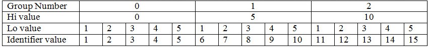
  select SEQ_ELECTRICITY_DEALS.NEXTVAL from dual; 

  If your network is not fast, this is definitely inefficient. Release 3.2.3 and later added an enhanced generator “SequenceStyleGenerator” along with 2 optimizers: hilo and pooled. Although they are covered in Chapter 5 “Basic O/R Mapping” in HRD the coverage is limited. Both optimizers use the HiLo algorithm. The algorithm generates an identifier equal to the Hi value plus the Lo value where the Hi value represents a group number and the Lo value sequentially and repeatedly iterates from 1 to the maximum group size. The group number will increase by 1 whenever the Lo value “clocks over” to 1.

  Suppose the group size is 5 (presented either by max_lo or increment_size parameter), here is an example:

  

  • Hilo optimizer
    The group number comes from the database sequence's next available value. The Hi value is defined in Hibernate as the Group Number multiplied by the increment_size parameter value.
  • Pooled optimizer
    The Hi value comes directly from the database sequence's next available value. Your database sequence should increment by the increment_size parameter value.

  Neither optimizer will hit the database until it has exhausted its in-memory group values. The above example hits the database every 5 identifier values. With the hilo optimizer, your sequence can't be used by other applications unless they also employ the same logic as in Hibernate. With the pooled optimizer, it is perfectly safe for other applications to use the same sequence.

  Both optimizers have a shortcoming. If Hibernate crashes, some of the identifier values in the current group may still be lost. However most applications don't require consecutive identifier values (If your database such as Oracle caches sequence values, you also lose identifier values if it crashes)

  If we use the pooled optimizer in example 11, here is the new id configuration:

  <id name = "key" column = " ID" >
      <generator class = "org.hibernate.id.enhance . SequenceStyleGenerator" >
          <param name = "sequence_name" > SEQ_ELECTRICITY_DEALS </param>
          <param name = "initial_value" > 0 </param>
          <param name = "increment_size" > 100 </param>
          <param name = "optimizer " > pooled </param>
      </generator>
  </id> 

  5 Summary

  This article covers most of the tuning skills you'll find helpful for your Hibernate application tuning. It allocates more time to tuning topics that are very efficient but poorly documented, such as inheritance mapping, second level cache and enhanced sequence identifier generators.

  It also mentions some database insights which are essential for tuning Hibernate.
  Some examples also contain practical solutions to problems you may encounter.

  Beyond this, it should be noted that Hibernate can work with In-Memory Data Grid (IMDG) such as Oracle's Coherance or GigaSpaces IMDG that can scale your application to milliseconds level.

  6 Resources

  [1] Latest Hibernate Reference Documentation on jboss.com

  [2] Oracle 9i Performance Tuning Guide and Reference

  [3] Performance Engineering on Wikipedia

  [4] Program Optimization on Wikipedia

  [5] Pareto Principle (the 80/20 rule) on Wikipedia

  [6] Premature Optimization on acm.org

  [7] Java Performance Tuning by Jack Shirazi

  [8] The Law of Leaky Abstractions by Joel Spolsky

  [9] Hibernate's StatisticsService Mbean configuration with Spring

  [10] JProbe by Quest Software

  [11] Java VisualVM

  [12] Column-oriented DBMS on Wikipedia

  [13] Apache DBCP BasicDataSource

  [14] JDBC Connection Pool by Oracle

  [15] Connection Failover by Oracle

  [16] Last Resource Commit Optimization (LRCO)

  [17] GigaSpaces for Hibernate ORM Users

  About the authors

  Yongjun Jiao is a technical manager at SunGard Consulting Services. He has been a professional software developer for the past 10 years. His expertise covers Java SE, Java EE, Oracle and application tuning. His recent focus has been on high performance computing including in-memory data grid, parallel and grid computing.

  Stewart Clark is a principal at SunGard Consulting Services. He has been a professional software developer and project manager for the past 15 years. His expertise covers core Java, Oracle and energy trading.

翻译自: https://www.infoq.com/articles/hibernate_tuning/?topicPageSponsorship=c1246725-b0a7-43a6-9ef9-68102c8d48e1