TensorFlow-形成图

TensorFlow-形成图 (TensorFlow - Forming Graphs)

A partial differential equation (PDE) is a differential equation, which involves partial derivatives with unknown function of several independent variables. With reference to partial differential equations, we will focus on creating new graphs.

偏微分方程(PDE)是一个微分方程，它涉及具有多个独立变量的未知函数的偏导数。 关于偏微分方程，我们将专注于创建新图。

Let us assume there is a pond with dimension 500*500 square −

让我们假设有一个尺寸为500 * 500平方的池塘-

N = 500

N = 500

Now, we will compute partial differential equation and form the respective graph using it. Consider the steps given below for computing graph.

现在，我们将计算偏微分方程并使用它形成相应的图。 考虑下面给出的计算图形的步骤。

Step 1 − Import libraries for simulation.

步骤1-导入库以进行仿真。

import tensorflow as tf
import numpy as np
import matplotlib.pyplot as plt

Step 2 − Include functions for transformation of a 2D array into a convolution kernel and simplified 2D convolution operation.

步骤2-包括用于将2D数组转换为卷积内核和简化2D卷积运算的函数。

def make_kernel(a):
   a = np.asarray(a)
   a = a.reshape(list(a.shape) + [1,1])
   return tf.constant(a, dtype=1)

def simple_conv(x, k):
   """A simplified 2D convolution operation"""
   x = tf.expand_dims(tf.expand_dims(x, 0), -1)
   y = tf.nn.depthwise_conv2d(x, k, [1, 1, 1, 1], padding = 'SAME')
   return y[0, :, :, 0]

def laplace(x):
   """Compute the 2D laplacian of an array"""
   laplace_k = make_kernel([[0.5, 1.0, 0.5], [1.0, -6., 1.0], [0.5, 1.0, 0.5]])
   return simple_conv(x, laplace_k)
   
sess = tf.InteractiveSession()

Step 3 − Include the number of iterations and compute the graph to display the records accordingly.

步骤3-包括迭代次数并计算图以相应地显示记录。

N = 500

# Initial Conditions -- some rain drops hit a pond

# Set everything to zero
u_init = np.zeros([N, N], dtype = np.float32)
ut_init = np.zeros([N, N], dtype = np.float32)

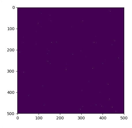
# Some rain drops hit a pond at random points
for n in range(100):
   a,b = np.random.randint(0, N, 2)
   u_init[a,b] = np.random.uniform()

plt.imshow(u_init)
plt.show()

# Parameters:
# eps -- time resolution
# damping -- wave damping
eps = tf.placeholder(tf.float32, shape = ())
damping = tf.placeholder(tf.float32, shape = ())

# Create variables for simulation state
U = tf.Variable(u_init)
Ut = tf.Variable(ut_init)

# Discretized PDE update rules
U_ = U + eps * Ut
Ut_ = Ut + eps * (laplace(U) - damping * Ut)

# Operation to update the state
step = tf.group(U.assign(U_), Ut.assign(Ut_))

# Initialize state to initial conditions
tf.initialize_all_variables().run()

# Run 1000 steps of PDE
for i in range(1000):
   # Step simulation
   step.run({eps: 0.03, damping: 0.04})
   
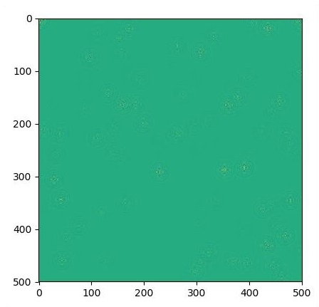
   # Visualize every 50 steps
   if i % 500 == 0:
      plt.imshow(U.eval())
      plt.show()

The graphs are plotted as shown below −

图形如下图所示-

翻译自: https://www.tutorialspoint.com/tensorflow/tensorflow_forming_graphs.htm