AI（009） - 词嵌入（Word Embedding）

本文链接：https://blog.csdn.net/darkrabbit/article/details/80823204

本文详细介绍了词嵌入的概念，探讨了词嵌入的局限性，并重点解析了word2vec模型，包括CBOW和skip-gram模型。同时，文章通过阅读tensorflow的word2vec_basic.py源码，逐步解释了模型的训练过程，帮助读者深入理解词嵌入的实战应用。

摘要生成于 C知道，由 DeepSeek-R1 满血版支持，前往体验 >

词嵌入（Word Embedding）

AI-第五期-DarkRabbit

这篇文章是对 Word Embedding 的一个总结，对应：

第十一周：（05）WordEmbedding_Attention
论文 arxiv 1301 .3781v3：Efficient Estimation of Word Representations in Vector Space
博客 colah’s blog：Deep Learning, NLP, and Representations
维基百科（en）：
tensorflow 官方教程（google）：word2vec
github word2vec_basic.py 源码：tensorflow/examples/tutorials/word2vec

公式在CSDN的app中会显示乱码，请在其它方式阅读

在卷积神经网络中，我们可以把词汇做 One Hot 编码，但这会造成我们的维度非常非常高。举例来说，在中文中就有6000多个二级常用字；而在英文中，单词数量是数十万，数百万的级别。这超大的维度显然限制了我们的运算速率。而且在 One Hot 中，彼此都是不互相关联的，这也不是我们需要的，在语言中，我们需要上下文等关系才能知道语意。

在 One Hot 中，我们把近似的词语都会加入训练，那么比如“番茄”与“西红柿”是一个意思，同样的东西为什么要用不同数据去训练呢？

综上所述，我们的一个解决办法就是使用分布式表示（Distributed representation），这样减小了我们的数据量。而这些多数是由人工来完成。

那么词嵌入（Word Embedding）就是代替我们人工来完成这项工作——学习到分布式表示（Distributed representation），在很多其它关于自然语言处理的论文中也同样都使用了它。

同样的还存在着，一个词语可有多种意义，比如一词多义。一个解决办法是意义嵌入（Sense embeddings）。

3 词嵌入模型（models）

经过上面的阐述，我们遇到的主要问题多数都是和“上下文（context）”有关，所以可以使用 word2vec 的方式，它可以利用两个模型体系结构中的任一个来产生词汇的分布式表示：continuous bag-of-words (CBOW) 与 continuous skip-gram 。

而这两个结构是由 [arxiv 1301 .3781v3] 提出。

new model architectures

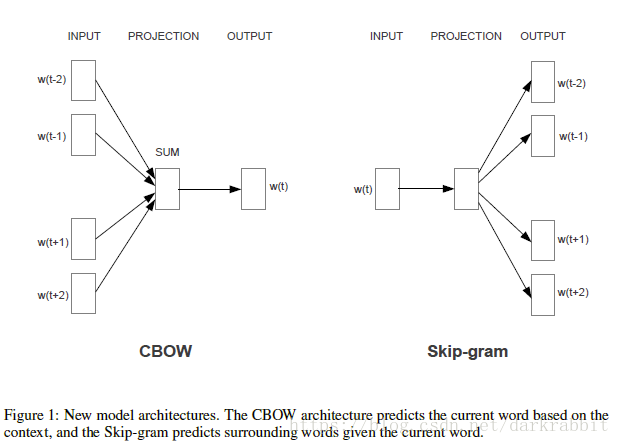
（图片来自 [arxiv 1301 .3781v3]）

对于它们来说，训练复杂度正比于：

O = E \times T \times Q

$O = E \times T \times Q$

其中 $E$ 是 training epochs 的数量， $T$ 是训练集中的词汇量数量， $Q$ 在接下来说明。

Continuous bag-of-words (CBOW)

这种方式将输入作为周边词，对中心词进行预测。

在输入层，使用 $1$ -of- $V$ 对 $N$ 前面的词进行编码， $V$ 是词汇量的大小。然后，使用一个共享的投影矩阵（projection matrix）将输入层投射到投影层（projection layer） $P$ ， $P$ 的维度是 $N \times D$ 。

Q = N \times D + D \times log 2 (V) (1)

$Q = N \times D + D \times \log_{2}(V) \quad (1)$

它和传统的 bag-of-words 有所不同，它使用上下文（context）的分布式表示（Distributed representation），并使用与NNLM同样的方式，来让输入层（input）和投影层（projection layer）的权重矩阵共享到所有词语的位置。

Continuous Skip-gram Model

这种方式将输入作为中心词，对周边词进行预测。

$Q = C \times (D + D \times log 2 (V)) (2)$ $Q = C \times (D + D \times \log_{2}(V)) \quad (2)$

其中， $C$ 是单词之间的最大距离。

[arxiv 1301 .3781v3]的原文描述

where $C$ is the maximum distance of the words. Thus, if we choose $C = 5$ , for each training word we will select randomly a number R in range $\left< 1;C \right>$ , and then use $R$ words from history and $R$ words from the future of the current word as correct labels. This will require us to do $R \times 2$ word classifications, with the current word as input, and each of the $R + R$ words as output. In the following experiments, we use $C = 10$ .

4 word2vec_basic.py 源码阅读

这是一个tensorflow中的简单例子，使用的是 Skip-gram 方式。

源码中，分为下列步骤：

下载与读取数据；
将词汇转换成字典映射（word - index）与反向映射（index - word），并将一些不常见词转换为“UNK”；
建立为模型（skip-gram model）生成训练 batch 的函数；
建立并训练 skip-gram 模型;
开始训练；
可视化。

可视化部分，不再进行介绍，关系不大；只是进行了结果输出成图片与图表的可视化。

4.1 下载与读取数据

这里只是定义了下载了数据与读取数据的函数。

唯一可说的就是读取数据时进行了分割。

# 数据地址
url = 'http://mattmahoney.net/dc/'

# 函数：下载数据
def maybe_download(filename, expected_bytes):
    ## 省略 source code

# 下载数据
filename = maybe_download('text8.zip', 31344016)

# 函数：读取数据
def read_data(filename):
    ## 省略 source code

# 读取数据（词汇量）
vocabulary = read_data(filename)

# 打印数据长度
print('Data size', len(vocabulary))

4.2 转换词汇成映射

# 定义取词汇量的数量
vocabulary_size = 50000

# 函数：建立新的数据集与映射
def build_dataset(words, n_words):
  """Process raw inputs into a dataset."""

  ## 词频列表
  ## 取词频最高的 vocabulary（50000）-1 个词，Index为0时，其它词数量（UNK）。
  count = [['UNK', -1]]
  count.extend(collections.Counter(words).most_common(n_words - 1))

  ## 生成映射（word - index）字典
  dictionary = dict()
  for word, _ in count:
    dictionary[word] = len(dictionary)

  ## 新的数据，并计算unk数量
  data = list()
  unk_count = 0
  for word in words:
    index = dictionary.get(word, 0)
    if index == 0:  # dictionary['UNK']
      unk_count += 1
    data.append(index)
  count[0][1] = unk_count

  ## 生成反向映射（index - word）字典
  reversed_dictionary = dict(zip(dictionary.values(), dictionary.keys()))

  ## 返回
  return data, count, dictionary, reversed_dictionary

# 建立新的数据集
data, count, dictionary, reverse_dictionary = build_dataset(
    vocabulary, vocabulary_size)

# 删除原始词汇量，并打印信息
del vocabulary  # Hint to reduce memory.
print('Most common words (+UNK)', count[:5])
print('Sample data', data[:10], [reverse_dictionary[i] for i in data[:10]])

4.3 generate_batch 函数

# 数据全局index
data_index = 0

# 函数：为 skip-grams 模型生成一个训练 batch（skip-grams是中心词作为输入）
  ## batch_size：每次读取多少数据（词 words）
  ## num_skips：word的重用次数
  ## skip_windows：为周围“上下文”取词的长度
    ### 举个例子：
    ### 比如取出的是 batch_value = “我是谁，我在哪，我在干什么”，num_skips = 2， skip_windows = 2
    ### 第一次取字后（“train label”）：“谁我”，“谁是”，“谁，”，“谁我”
      #### 每次只取左（右）中的2个字（skip_windows）
    ### 从取字后，再随机从中取 num_skips 个：“谁我”，“谁，”（假设取了这俩）
      #### 输入（中心词）用了2次（num_skips）
    ### 第二次取字后（“train label”）：“，我”，“，是”，“，谁”，“，我”
    ### 直到循环结束
def generate_batch(batch_size, num_skips, skip_window):

  ## 声明使用全局 data_index
  global data_index

  ## 断言
  assert batch_size % num_skips == 0
  assert num_skips <= 2 * skip_window

  ## 构造 batch 与 labels，为其分配空间
  batch = np.ndarray(shape=(batch_size), dtype=np.int32)
  labels = np.ndarray(shape=(batch_size, 1), dtype=np.int32)

  ## 上下文与中心词的总长度
  span = 2 * skip_window + 1  # [ skip_window target skip_window ]

  ## 缓冲区，双端队列（最大长度 span）
  buffer = collections.deque(maxlen=span)  # pylint: disable=redefined-builtin

  ## 如果全部数据已经读取完成，重新从0开始读取
  if data_index + span > len(data):
    data_index = 0

  ## 将上下文与中心词加入到缓冲区
  buffer.extend(data[data_index:data_index + span])

  ## 每次读取 span 个词
  data_index += span

  ## 循环遍历
  for i in range(batch_size // num_skips):
    ### 取上下文
    context_words = [w for w in range(span) if w != skip_window]
    ### 在上下文中，随机取 num_skips 的词
    words_to_use = random.sample(context_words, num_skips)
    ### 将 中心词 与 上下文，加入到 batch 与 labels中
    for j, context_word in enumerate(words_to_use):
      batch[i * num_skips + j] = buffer[skip_window]
      labels[i * num_skips + j, 0] = buffer[context_word]
    ### 如果全部数据已经读取完成，重新读取最初的 span 个词
    if data_index == len(data):
      buffer.extend(data[0:span])
      data_index = span
    ### 如果没有读取完成，将下一个词放去缓冲区中，将首个词移除队列
    else:
      buffer.append(data[data_index])
      data_index += 1
  # Backtrack a little bit to avoid skipping words in the end of a batch
  data_index = (data_index + len(data) - span) % len(data)
  return batch, labels

# 为 skip-grams 模型生成一个训练 batch 与 labels
batch, labels = generate_batch(batch_size=8, num_skips=2, skip_window=1)
# 打印前8个
for i in range(8):
  print(batch[i], reverse_dictionary[batch[i]], '->', labels[i, 0],
        reverse_dictionary[labels[i, 0]])

4.4 建立并训练skip-gram模型

# 训练参数
batch_size = 128
embedding_size = 128  # Dimension of the embedding vector.
skip_window = 1  # How many words to consider left and right.
num_skips = 2  # How many times to reuse an input to generate a label.
num_sampled = 64  # Number of negative examples to sample.

# 验证参数
valid_size = 16  # Random set of words to evaluate similarity on.
valid_window = 100  # Only pick dev samples in the head of the distribution.
valid_examples = np.random.choice(valid_window, valid_size, replace=False)

# 构造一个新图
graph = tf.Graph()

with graph.as_default():
  ## 输入占位
  with tf.name_scope('inputs'):
    train_inputs = tf.placeholder(tf.int32, shape=[batch_size])
    train_labels = tf.placeholder(tf.int32, shape=[batch_size, 1])
    valid_dataset = tf.constant(valid_examples, dtype=tf.int32)

  ## 使用CPU进行嵌入
  with tf.device('/cpu:0'):

    ### 对输入进行 Look up embeddings
    with tf.name_scope('embeddings'):
      embeddings = tf.Variable(
          tf.random_uniform([vocabulary_size, embedding_size], -1.0, 1.0))
      embed = tf.nn.embedding_lookup(embeddings, train_inputs)

    ### 构造 NCE loss 的变量
    with tf.name_scope('weights'):
      nce_weights = tf.Variable(
          tf.truncated_normal(
              [vocabulary_size, embedding_size],
              stddev=1.0 / math.sqrt(embedding_size)))

    ### 添加偏置
    with tf.name_scope('biases'):
      nce_biases = tf.Variable(tf.zeros([vocabulary_size]))

  ## 平均 NCE loss
  with tf.name_scope('loss'):
    loss = tf.reduce_mean(
        tf.nn.nce_loss(
            weights=nce_weights,
            biases=nce_biases,
            labels=train_labels,
            inputs=embed,
            num_sampled=num_sampled,
            num_classes=vocabulary_size))

  # Add the loss value as a scalar to summary.
  tf.summary.scalar('loss', loss)

  # 构造 SGD optimizer
  with tf.name_scope('optimizer'):
    optimizer = tf.train.GradientDescentOptimizer(1.0).minimize(loss)

  # minibatch 样本与所有 embeddings 的余弦相似度
  norm = tf.sqrt(tf.reduce_sum(tf.square(embeddings), 1, keepdims=True))
  normalized_embeddings = embeddings / norm
  valid_embeddings = tf.nn.embedding_lookup(normalized_embeddings,
                                            valid_dataset)
  similarity = tf.matmul(
      valid_embeddings, normalized_embeddings, transpose_b=True)

  # 合并所有 summaries.
  merged = tf.summary.merge_all()

  # Add variable initializer.
  init = tf.global_variables_initializer()

  # Create a saver.
  saver = tf.train.Saver()

4.5 开始训练

# 训练 steps
num_steps = 100001

with tf.Session(graph=graph) as session:
  # Open a writer to write summaries.
  writer = tf.summary.FileWriter(FLAGS.log_dir, session.graph)

  # We must initialize all variables before we use them.
  init.run()
  print('Initialized')

  average_loss = 0
  for step in xrange(num_steps):
    ### 为 skip-grams 模型生成一个训练 batch
    batch_inputs, batch_labels = generate_batch(batch_size, num_skips,
                                                skip_window)
    feed_dict = {train_inputs: batch_inputs, train_labels: batch_labels}

    # Define metadata variable.
    run_metadata = tf.RunMetadata()

    ### 运行优化器、合并和loss
    _, summary, loss_val = session.run(
        [optimizer, merged, loss],
        feed_dict=feed_dict,
        run_metadata=run_metadata)
    average_loss += loss_val

    # Add returned summaries to writer in each step.
    writer.add_summary(summary, step)

    # Add metadata to visualize the graph for the last run.
    if step == (num_steps - 1):
      writer.add_run_metadata(run_metadata, 'step%d' % step)

    ### 每2000个steps，打印一次loss
    if step % 2000 == 0:
      if step > 0:
        average_loss /= 2000
      # The average loss is an estimate of the loss over the last 2000 batches.
      print('Average loss at step ', step, ': ', average_loss)
      average_loss = 0

    ### 每10000个steps，验证一次，并打印
    # Note that this is expensive (~20% slowdown if computed every 500 steps)
    if step % 10000 == 0:
      sim = similarity.eval()
      for i in xrange(valid_size):
        valid_word = reverse_dictionary[valid_examples[i]]
        top_k = 8  # number of nearest neighbors
        nearest = (-sim[i, :]).argsort()[1:top_k + 1]
        log_str = 'Nearest to %s:' % valid_word
        for k in xrange(top_k):
          close_word = reverse_dictionary[nearest[k]]
          log_str = '%s %s,' % (log_str, close_word)
        print(log_str)

  ## 最终 embeddings
  final_embeddings = normalized_embeddings.eval()

  ## 保存 embeddings 的反向映射.
  with open(FLAGS.log_dir + '/metadata.tsv', 'w') as f:
    for i in xrange(vocabulary_size):
      f.write(reverse_dictionary[i] + '\n')

  # 保存模型的 checkpoints.
  saver.save(session, os.path.join(FLAGS.log_dir, 'model.ckpt'))

  # 在 TensorBoard 建立可视化参数.
  config = projector.ProjectorConfig()
  embedding_conf = config.embeddings.add()
  embedding_conf.tensor_name = embeddings.name
  embedding_conf.metadata_path = os.path.join(FLAGS.log_dir, 'metadata.tsv')
  projector.visualize_embeddings(writer, config)

writer.close()