


正常情况下,数据库只会按单列收集统计信息,无法捕捉到任何关于跨列的相关性信息。扩展统计信息是从10版本引入,可以通过命令 CREATE STATISTICS 创建多列相关的统计信息。
因为一个表一般有多个列,多列的任意组合很大,所以自动收集多列统计信息不现实,而我们可以根据自己的需求自己来创建多列的统计信息,这样可以让相关查询执行计划更加准确。
下面举例介绍几种扩展统计的几种类型:
- Functional Dependencies
- Multivariate N-Distinct Counts
- Multivariate MCV Lists (12版本引入)
以下示例均在13.4版本测试
Functional Dependencies实例
#创建测试表,并插入数据
CREATE TABLE expenses(
   pk int GENERATED ALWAYS AS IDENTITY,
   value money,
   day date,
   quarter int,
   year int,
   incoming boolean DEFAULT false,
   account  text DEFAULT 'cash',
   PRIMARY KEY ( pk ),
   CHECK( value <> 0::money ),
   CHECK( quarter = EXTRACT( quarter FROM day ) ),
   CHECK( year = EXTRACT( year FROM day ) )
);
#上面quarter和year字段均依赖字段day的值,当value字段大于0时,incoming字段为TRUE,否则为false.
#因为列之间有关系,我们创建相关的触发器和触发器函数
CREATE OR REPLACE FUNCTION f_expenses()
RETURNS TRIGGER
AS $code$
BEGIN
  IF NEW.day IS NULL THEN
     NEW.day := CURRENT_DATE;
  END IF;

  IF NEW.value = 0::money THEN
     NEW.value := 0.01::money;
  END IF;

  NEW.quarter  := EXTRACT( quarter FROM NEW.day );
  NEW.year     := EXTRACT( year FROM NEW.day );
  IF NEW.value > 0::money THEN
     NEW.incoming := true;
  ELSE
    NEW.incoming := false;
  END IF;

  RETURN NEW;
END
$code$
LANGUAGE plpgsql;

CREATE TRIGGER tr_expenses BEFORE INSERT OR UPDATE ON expenses
FOR EACH ROW
EXECUTE PROCEDURE f_expenses();

#插入测试数据
WITH v(value, counter, account) AS (
   SELECT ( random() * 100 )::numeric + 1 * CASE v % 2 WHEN 0 THEN 1 ELSE -1 END,
          v,
          CASE v % 3 WHEN 0 THEN 'credit card'
                     WHEN 1 THEN 'bank'
                     ELSE 'cash'
         END
  FROM generate_series( 1, 2000000 ) v
)

INSERT INTO expenses( value, day, account )
SELECT value, CURRENT_DATE - ( counter % 1000 ), account
FROM v;

SELECT
 count(*) FILTER( WHERE year = 2019 ) AS total_2016_by_year,
 count(*) FILTER( WHERE EXTRACT( year FROM day ) = 2019 ) AS total_2019_by_day,
 count(*) FILTER( WHERE year = 2019 AND incoming = true AND day = '2019-7-19'::date ) AS incoming_by_year,
 count(*) FILTER( WHERE EXTRACT( year FROM day ) = 2019 AND incoming = true AND day = '2019-7-19'::date ) AS incoming_2019_by_day,
 pg_size_pretty( pg_relation_size( 'expenses' ) ) AS table_size
 FROM expenses;

 total_2016_by_year | total_2019_by_day | incoming_by_year | incoming_2019_by_day | table_size
--------------------+-------------------+------------------+----------------------+------------
             488000 |            488000 |             1988 |                 1988 | 136 MB


#这里执行同样条件的查询,,执行计划评估为480行,明显和上面的1988相差很远
EXPLAIN
SELECT count(*)
FROM expenses
WHERE incoming = true
AND   value > 0.0::money
AND   day = '2019-7-19'::date
AND   year = 2019;
                                               QUERY PLAN
--------------------------------------------------------------------------------------------------------
 Gather  (cost=1000.00..35106.67 rows=480 width=32)
   Workers Planned: 2
   ->  Parallel Seq Scan on expenses  (cost=0.00..34058.67 rows=200 width=32)
         Filter: (incoming AND (day = '2019-07-19'::date) AND (year = 2019) AND (value > (0.0)::money))
(4 rows)

#创建相关扩展统计信息
CREATE STATISTICS stat_day_year ( dependencies )
 ON day, year
 FROM expenses;

CREATE STATISTICS stat_day_quarter ( dependencies )
 ON day, quarter
 FROM expenses;

CREATE STATISTICS stat_value_incoming( dependencies )
 ON value, incoming
 FROM expenses;

#分析后拿到最新的统计信息,查看依赖关系
#可见4(quarter)和5(year)通过函数{f}依赖于3(day),6(incoming)依赖于2(value)
analyze;

SELECT s.stxrelid::regclass AS table_name,
       s.stxname AS statistics_name,
       d.stxdndistinct AS ndistinct,
       d.stxddependencies AS dependencies
FROM pg_statistic_ext AS s
   JOIN pg_statistic_ext_data AS d
      ON d.stxoid = s.oid;

 table_name |   statistics_name   |   ndistinct    |     dependencies
------------+---------------------+----------------+----------------------
 expenses   | stat_day_year       |                | {"3 => 5": 1.000000}
 expenses   | stat_day_quarter    |                | {"3 => 4": 1.000000}
 expenses   | stat_value_incoming |                | {"2 => 6": 1.000000}
#再次执行查看执行计划评估为1972行,明显比刚才的评估更加精准
EXPLAIN
SELECT count(*)
FROM expenses
WHERE incoming = true
AND   value > 0.0::money
AND   day = '2019-7-19'::date
AND   year = 2019;

                                               QUERY PLAN
--------------------------------------------------------------------------------------------------------
 Gather  (cost=1000.00..35255.87 rows=1972 width=32)
   Workers Planned: 2
   ->  Parallel Seq Scan on expenses  (cost=0.00..34058.67 rows=822 width=32)
         Filter: (incoming AND (day = '2019-07-19'::date) AND (year = 2019) AND (value > (0.0)::money))
(4 rows)

#查看一下,确实是1988
SELECT count(*)
FROM expenses
WHERE incoming = true
AND   value > 0.0::money
AND   day = '2019-7-19'::date
AND   year = 2019;

 count
-------
  1988
(1 row)
Multivariate N-Distinct Counts实例
该类型在分组聚合的时候可以使得执行计划更加准确,不准确评估,可能会导致差的执行计划,实例如下:
#建表,插入数据,分析表,查看执行计划
CREATE TABLE tbl (
    col1 int,
    col2 int
);

INSERT INTO tbl SELECT i/10000, i/100000
FROM generate_series (1,10000000) s(i);

ANALYZE tbl;
#关闭并行
postgres=# SET max_parallel_workers_per_gather TO 0;
SET
#可建执行计划评估的rows=100000
EXPLAIN ANALYZE SELECT col1,col2,count(*) from tbl group by col1, col2;
                                                      QUERY PLAN
-----------------------------------------------------------------------------------------------------------------------
 HashAggregate  (cost=731746.42..810871.24 rows=100000 width=16) (actual time=2101.286..2101.651 rows=1001 loops=1)
   Group Key: col1, col2
   Planned Partitions: 4  Batches: 1  Memory Usage: 1681kB
   ->  Seq Scan on tbl  (cost=0.00..144247.77 rows=9999977 width=8) (actual time=0.029..637.266 rows=10000000 loops=1)
 Planning Time: 0.138 ms
 Execution Time: 2101.891 ms
(6 rows)

#创建STATISTICS来捕获n_distinct类型的统计信息,然后再次执行
postgres=# CREATE STATISTICS s2 (ndistinct) on col1, col2 from tbl;
CREATE STATISTICS

postgres=# analyze tbl ;
ANALYZE

#可见rows=1000,执行计划评估更加准确,
postgres=# EXPLAIN ANALYZE SELECT col1,col2,count(*) from tbl group by col1, col2;
                                                      QUERY PLAN
-----------------------------------------------------------------------------------------------------------------------
 HashAggregate  (cost=219247.60..219257.60 rows=1000 width=16) (actual time=2130.718..2130.863 rows=1001 loops=1)
   Group Key: col1, col2
   Batches: 1  Memory Usage: 193kB
   ->  Seq Scan on tbl  (cost=0.00..144247.77 rows=9999977 width=8) (actual time=0.020..637.584 rows=10000000 loops=1)
 Planning Time: 0.107 ms
 Execution Time: 2130.930 ms
(6 rows)


#查看扩展统计信息,查看s2
 SELECT s.stxrelid::regclass AS table_name,
        s.stxname AS statistics_name,
        d.stxdndistinct AS ndistinct,
        d.stxddependencies AS dependencies
 FROM pg_statistic_ext AS s
    JOIN pg_statistic_ext_data AS d
       ON d.stxoid = s.oid;
 table_name |   statistics_name   |   ndistinct    |     dependencies
------------+---------------------+----------------+----------------------
 expenses   | stat_day_year       |                | {"3 => 5": 1.000000}
 expenses   | stat_day_quarter    |                | {"3 => 4": 1.000000}
 expenses   | stat_value_incoming |                | {"2 => 6": 1.000000}
 tbl        | s2                  | {"1, 2": 1000} |
#这里可见stxkind类型为{d}
postgres=# select * from pg_statistic_ext where stxname='s2';
  oid  | stxrelid | stxname | stxnamespace | stxowner | stxstattarget | stxkeys | stxkind
-------+----------+---------+--------------+----------+---------------+---------+---------
 16707 |    16704 | s2      |         2200 |       10 |            -1 | 1 2     | {d}
Multivariate MCV Lists实例
#创建表,插入数据,并创建mcv类型的扩展统计信息
postgres=# create table tbl_mcv(c1 int, c2 int, c3 int);
CREATE TABLE

postgres=# insert into tbl_mcv select random()*10, random()*20, random()*30 from generate_series(1,100000);
INSERT 0 100000

postgres=# insert into tbl_mcv select random()*10, random()*20, 1 from generate_series(1,100000);
INSERT 0 100000

postgres=# create statistics st1 (mcv) on c1,c2,c3 from tbl_mcv;
CREATE STATISTICS
postgres=#analyze tbl_mcv;
ANALYZE

#这里可见stxkind为{m}
postgres=#  select * from pg_statistic_ext where stxname='st1';
  oid  | stxrelid | stxname | stxnamespace | stxowner | stxstattarget | stxkeys | stxkind
-------+----------+---------+--------------+----------+---------------+---------+---------
 16716 |    16713 | st1     |         2200 |       10 |            -1 | 1 2 3   | {m}


 postgres=# select pg_mcv_list_items(stxdmcv)from pg_statistic_ext_data ;
                           pg_mcv_list_items
-----------------------------------------------------------------------
 (0,"{9,9,1}","{f,f,f}",0.0036,0.0027182991080000004)
 (1,"{7,3,1}","{f,f,f}",0.0034,0.0026549472754444445)
 (2,"{2,2,1}","{f,f,f}",0.0033666666666666667,0.0026956065623703705)
 (3,"{2,13,1}","{f,f,f}",0.003266666666666667,0.002661822575111111)
 (4,"{1,6,1}","{f,f,f}",0.0032333333333333333,0.002674537851333333)
 (5,"{6,15,1}","{f,f,f}",0.0032333333333333333,0.002655599209037037)
 (6,"{8,2,1}","{f,f,f}",0.0032,0.002642768516)
 (7,"{6,6,1}","{f,f,f}",0.0032,0.0026470657925555556)
 (8,"{3,14,1}","{f,f,f}",0.0032,0.0026162992122222223)
 (9,"{3,5,1}","{f,f,f}",0.0032,0.0026469989422222224)
 (10,"{5,3,1}","{f,f,f}",0.0031666666666666666,0.002542249612222222)
 (11,"{1,18,1}","{f,f,f}",0.0031333333333333335,0.0026245303737777773)
 (12,"{6,18,1}","{f,f,f}",0.0031,0.0025975719769629627)
 (13,"{3,6,1}","{f,f,f}",0.0031,0.002645293401666667)
 (14,"{1,2,1}","{f,f,f}",0.003033333333333333,0.0026141839991111106)
 (15,"{4,16,1}","{f,f,f}",0.003,0.0025546923447777774)
 (16,"{1,13,1}","{f,f,f}",0.003,0.002581420479333333)
 (17,"{2,5,1}","{f,f,f}",0.0029666666666666665,0.0027596183277037037)
 (18,"{4,14,1}","{f,f,f}",0.0029333333333333334,0.002597016604962963)
 (19,"{1,12,1}","{f,f,f}",0.0029333333333333334,0.0025917668539999997)
 (20,"{5,6,1}","{f,f,f}",0.0029,0.0025788287433333333)
 (21,"{4,17,1}","{f,f,f}",0.0029,0.002514061055)
 (22,"{5,4,1}","{f,f,f}",0.0029,0.0024807301644444446)
 (23,"{2,14,1}","{f,f,f}",0.0029,0.002727612445037037)
 (24,"{7,4,1}","{f,f,f}",0.0029,0.0025907006768888887)
 (25,"{8,3,1}","{f,f,f}",0.0029,0.002665430779)
 (26,"{5,19,1}","{f,f,f}",0.0028666666666666667,0.0025156466077777776)
 (27,"{6,16,1}","{f,f,f}",0.0028666666666666667,0.002575385094111111)
 (28,"{4,3,1}","{f,f,f}",0.0028666666666666667,0.002588551752925926)
 (29,"{8,14,1}","{f,f,f}",0.0028666666666666667,0.002674147034)
 (30,"{9,10,1}","{f,f,f}",0.0028666666666666667,0.0025950556618518517)
 (31,"{9,3,1}","{f,f,f}",0.0028333333333333335,0.0026540736501481483)
 (32,"{6,4,1}","{f,f,f}",0.0028333333333333335,0.0025463714780740738)
 (33,"{6,12,1}","{f,f,f}",0.0028333333333333335,0.002565144994333333)
 (34,"{2,10,1}","{f,f,f}",0.0028,0.0026582663659259257)
 (35,"{2,8,1}","{f,f,f}",0.0028,0.002549801985777778)
 (36,"{4,9,1}","{f,f,f}",0.0028,0.002651191658)
 (37,"{6,19,1}","{f,f,f}",0.0028,0.0025822118272962958)
 (38,"{4,10,1}","{f,f,f}",0.0028,0.002530990759074074)
 (39,"{3,11,1}","{f,f,f}",0.002766666666666667,0.0025412554277777777)
 (40,"{7,9,1}","{f,f,f}",0.002766666666666667,0.002719193874)
 (41,"{8,18,1}","{f,f,f}",0.002766666666666667,0.0026532280219999996)
 (42,"{7,16,1}","{f,f,f}",0.002766666666666667,0.0026202193843333334)
 (43,"{7,1,1}","{f,f,f}",0.002766666666666667,0.002418797615888889)
 (44,"{8,10,1}","{f,f,f}",0.0027333333333333333,0.002606160245)
 (45,"{2,7,1}","{f,f,f}",0.0027333333333333333,0.002596032705185185)
 (46,"{1,15,1}","{f,f,f}",0.0027333333333333333,0.002683159830222222)
 (47,"{8,5,1}","{f,f,f}",0.0027333333333333333,0.002705525552)
 (48,"{1,19,1}","{f,f,f}",0.0027333333333333333,0.0026090108117777775)
 (49,"{3,19,1}","{f,f,f}",0.0027333333333333333,0.0025804828605555555)
 (50,"{2,9,1}","{f,f,f}",0.0027333333333333333,0.0027845117920000002)
 (51,"{7,11,1}","{f,f,f}",0.0027333333333333333,0.002587227887777778)
 (52,"{8,9,1}","{f,f,f}",0.0027333333333333333,0.002729931066)
 (53,"{2,19,1}","{f,f,f}",0.0027333333333333333,0.0026902722485925923)
 (54,"{2,16,1}","{f,f,f}",0.0027333333333333333,0.002683159830222222)
 (55,"{9,1,1}","{f,f,f}",0.0027,0.002418001696962963)
 (56,"{2,4,1}","{f,f,f}",0.0027,0.002652932052148148)
 (57,"{6,17,1}","{f,f,f}",0.0027,0.0025344246950000002)
 (58,"{9,7,1}","{f,f,f}",0.0027,0.00253430185037037)
 (59,"{2,12,1}","{f,f,f}",0.0027,0.002672491202666667)
 (60,"{4,7,1}","{f,f,f}",0.0027,0.0024717367948148146)
 (61,"{7,12,1}","{f,f,f}",0.0027,0.0026098010169999996)
 (62,"{7,6,1}","{f,f,f}",0.0027,0.0026931479556666664)
 (63,"{3,13,1}","{f,f,f}",0.0027,0.0025531942116666668)
 (64,"{8,13,1}","{f,f,f}",0.0027,0.002609646747)
 (65,"{2,18,1}","{f,f,f}",0.0027,0.0027062751899259254)
 (66,"{9,14,1}","{f,f,f}",0.0026666666666666666,0.0026627527660740744)
 (67,"{5,9,1}","{f,f,f}",0.0026666666666666666,0.0026037690600000003)
 (68,"{1,1,1}","{f,f,f}",0.0026666666666666666,0.002402083318444444)
 (69,"{9,5,1}","{f,f,f}",0.0026666666666666666,0.0026939975834074075)
 (70,"{6,14,1}","{f,f,f}",0.0026666666666666666,0.002618052176518518)
 (71,"{3,10,1}","{f,f,f}",0.0026333333333333334,0.0025497831305555554)
 (72,"{8,4,1}","{f,f,f}",0.0026333333333333334,0.0026009304919999998)
 (73,"{7,2,1}","{f,f,f}",0.0026333333333333334,0.002632374146222222)
 (74,"{4,18,1}","{f,f,f}",0.0026333333333333334,0.0025767009600740744)
 (75,"{4,12,1}","{f,f,f}",0.0026333333333333334,0.002544534522333333)
 (76,"{7,15,1}","{f,f,f}",0.0026333333333333334,0.0027018299284444444)
 (77,"{5,15,1}","{f,f,f}",0.0026333333333333334,0.0025871421822222223)
 (78,"{7,14,1}","{f,f,f}",0.0026333333333333334,0.002663629248222222)
 (79,"{1,14,1}","{f,f,f}",0.0026333333333333334,0.002645223123111111)
 (80,"{9,19,1}","{f,f,f}",0.0026333333333333334,0.0026263004791851853)
 (81,"{1,3,1}","{f,f,f}",0.0026333333333333334,0.002636601144222222)
 (82,"{6,5,1}","{f,f,f}",0.0026,0.0026487724758518516)
 (83,"{7,18,1}","{f,f,f}",0.0026,0.0026427925135555554)
 (84,"{6,10,1}","{f,f,f}",0.0026,0.0025514915279629628)
 (85,"{8,19,1}","{f,f,f}",0.0026,0.0026375387629999996)
 (86,"{3,17,1}","{f,f,f}",0.0026,0.0025327277250000004)
 (87,"{8,12,1}","{f,f,f}",0.0025666666666666667,0.0026201062529999995)
 (88,"{3,4,1}","{f,f,f}",0.0025666666666666667,0.0025446665088888886)
 (89,"{5,5,1}","{f,f,f}",0.0025666666666666667,0.002580491431111111)
 (90,"{1,10,1}","{f,f,f}",0.0025666666666666667,0.0025779716877777775)
 (91,"{1,5,1}","{f,f,f}",0.0025666666666666667,0.002676262247111111)
 (92,"{6,7,1}","{f,f,f}",0.002533333333333333,0.0024917576125925924)
 (93,"{4,2,1}","{f,f,f}",0.002533333333333333,0.0025665431376296296)
 (94,"{7,19,1}","{f,f,f}",0.002533333333333333,0.002627164962555555)
 (95,"{8,6,1}","{f,f,f}",0.002533333333333333,0.002703782301)
 (96,"{9,6,1}","{f,f,f}",0.002533333333333333,0.0026922617602222225)
 (97,"{9,8,1}","{f,f,f}",0.002533333333333333,0.0024891704475555557)
 (98,"{6,9,1}","{f,f,f}",0.002533333333333333,0.002672666042)
 (99,"{8,16,1}","{f,f,f}",0.002533333333333333,0.0026305657589999996)

#以上说明有100种不同的组合,以及出现的频率,和基于单列统计信息的基本频率。PG默认是100个桶,如果觉的需要更精准,可以增加default_statistics_target (integer)参数的值,同时也会增加analyze的时间。
#和Functional Dependencies不同的有两点,
#第一,MCV的list存储实际的值,从而决定了那些组合是兼容的,如下
postgres=# EXPLAIN (ANALYZE, TIMING OFF) SELECT * FROM tbl_mcv WHERE c1 = 1 AND c2 = 10;
                                       QUERY PLAN
----------------------------------------------------------------------------------------
 Seq Scan on tbl_mcv  (cost=0.00..4082.00 rows=1000 width=12) (actual rows=984 loops=1)
   Filter: ((c1 = 1) AND (c2 = 10))
   Rows Removed by Filter: 199016
 Planning Time: 0.086 ms
 Execution Time: 11.532 ms
(5 rows)

#第二,MCV可以处理范围子句,而不仅仅是等值类型的判断,如下
postgres=# EXPLAIN (ANALYZE, TIMING OFF) select * from tbl_mcv WHERE c1 < 5 AND c2 > 5;
                                        QUERY PLAN
-------------------------------------------------------------------------------------------
 Seq Scan on tbl_mcv  (cost=0.00..4082.00 rows=67033 width=12) (actual rows=65199 loops=1)
   Filter: ((c1 < 5) AND (c2 > 5))
   Rows Removed by Filter: 134801
 Planning Time: 0.057 ms
 Execution Time: 13.610 ms
(5 rows)
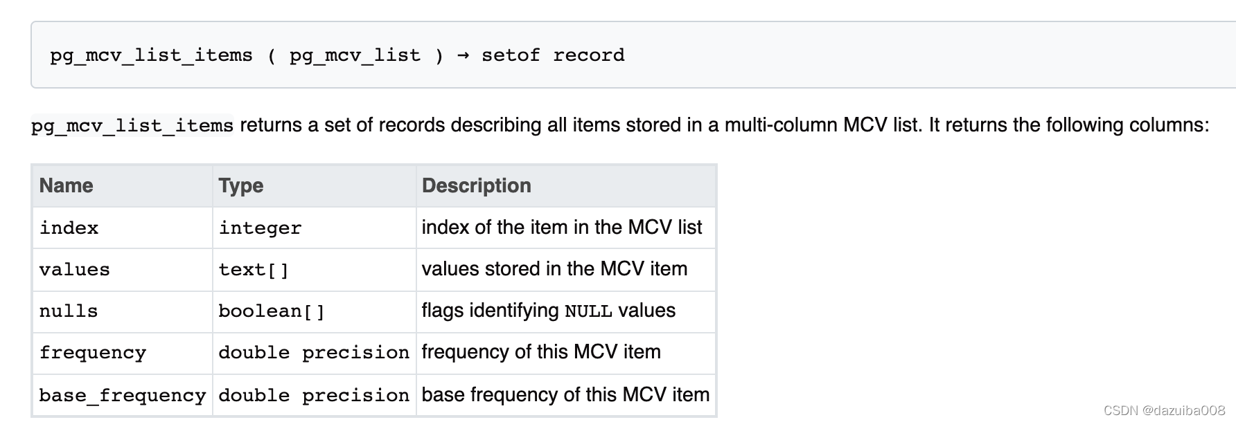
pg_mcv_list_item解释:
这里其字段比较好理解,主要说下frequency和base_frequency,frequency表示该条目的出现频率,base_frequency是根据单列的统计信息计算的频率,好比没有多列的统计信息。如:
(0,"{9,9,1}","{f,f,f}",0.0036,0.0027182991080000004)
0表示MCV list的索引号,{9,9,1}表示存储在MCV列表的值,{f,f,f}表示是否为空值,如果是null,则相应值为t,0.0036表示该条目在MCV中的频率,base_frequency则表示根据单列统计信息计算的基础频率。
扩展统计信息相关视图:
pg_stats_ext
pg_statistic_ext
pg_statistic_ext_data
源码相关:
src/backend/statistics/mcv.c
src/backend/statistics/mvdistinct.c
src/backend/statistics/dependencies.c
参考:
https://www.postgresql.org/docs/13/planner-stats.html#PLANNER-STATS-EXTENDED
https://www.postgresql.org/docs/current/multivariate-statistics-examples.html
https://github.com/digoal/blog/blob/master/201903/20190330_05.md
https://github.com/digoal/blog/blob/master/201709/20170902_02.md
https://fluca1978.github.io/2018/06/28/PostgreSQLExtendedStatistics.html


 181
181


 被折叠的 条评论
为什么被折叠?
被折叠的 条评论
为什么被折叠?
 到【灌水乐园】发言


