深度学习基础（三）（稀疏）自编码器分类：深度学习 ...

最新推荐文章于 2024-01-08 01:28:52 发布

dengxundong1074

最新推荐文章于 2024-01-08 01:28:52 发布

阅读量1k

点赞数

文章标签：人工智能 php

原文链接：http://www.cnblogs.com/learnordie/p/4656966.html

版权

我们知道在神经网络上通过前向传导和后向传导算法，可以再给定训练集的基础上训练参数，这是神经网络有监督学习的一种应用。但是有时候数据集并不是都有标签的，我们希望给一堆数据之后，通过神经网络，在没有既定目标函数的情况下，在一定约束下神经网络能够自行独立地学习到一些参数。这种没有特定学习目标的学习方法，就叫做无监督的学习方法。

现在来看一种最简单的无监督神经网络算法，自编码器。

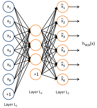
自编码器神经网络是一种运用后向传递算的无监督的算法。

给定一系列无监督的训练集 $\textstyle \{x^{(1)}, x^{(2)}, x^{(3)}, \ldots\}$ $\textstyle x^{(i)} \in \Re^{n}$

初始化的时，令 $\textstyle y^{(i)} = x^{(i)}$

我们希望经过训练后： $\textstyle h_{W,b}(x) \approx x$

这实际上是学习了一个单位函数。单位函数很常见的，只是单位函数本身作用是有限的，自编码神经网络的精髓在于中间的隐层，通过对中间隐层的约束，我们可以得到很多有用的结果。我们接下来讨论两个常见的约束：

1.隐层单元个数小于输入层单元个数

这个时候中间隐层相当于降维。

2.隐层单元个数大于输入层单元个数，这个时候我们可以加入稀疏约束，中间隐层是一组稀疏向量

我们现在着重讨论第二个约束，也就是稀疏自编码器。

首先，我们假设一个单元被激活当且仅当它的输出值接近1，不被激活当它的输出值接近0.（默认激活函数为sigmod函数）

$\textstyle a^{(2)}_j$ ：代表的是隐层的第j个单元

特别地，在这里我们用 $\textstyle a^{(2)}_j(x)$ 表示这个单元被激活，如果

$\begin{align}\sum_{j=1}^{s_2} \rho \log \frac{\rho}{\hat\rho_j} + (1-\rho) \log \frac{1-\rho}{1-\hat\rho_j}.\end{align}$

$\begin{align}\hat\rho_j = \frac{1}{m} \sum_{i=1}^m \left[ a^{(2)}_j(x^{(i)}) \right]\end{align}$

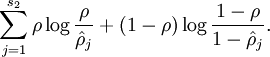
我们将稀疏约束的数学形式给出：

$\begin{align}\hat\rho_j = \rho,\end{align}$

其中 $\textstyle \rho$ 表示稀疏参数，一般是0.05

这个稀疏约束的意思就是中间隐层的大部分单元都是未被激活的（输出值接近0）

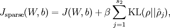
现在我们需要得出稀疏自编码的代价函数，这个代价函数很显然要考虑到稀疏约束这个条件，因此我们引入：

$\begin{align}\sum_{j=1}^{s_2} \rho \log \frac{\rho}{\hat\rho_j} + (1-\rho) \log \frac{1-\rho}{1-\hat\rho_j}.\end{align}$

也就是：

$\begin{align}\sum_{j=1}^{s_2} {\rm KL}(\rho || \hat\rho_j),\end{align}$

$\textstyle {\rm KL}(\rho || \hat\rho_j) = \rho \log \frac{\rho}{\hat\rho_j} + (1-\rho) \log \frac{1-\rho}{1-\hat\rho_j}$

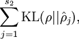
KL距离，是Kullback-Leibler差异（Kullback-Leibler Divergence）的简称，也叫做相对熵（Relative Entropy）。它衡量的是相同事件空间里的两个概率分布的差异情况。我们在这里只需要知道 $\begin{align}\hat\rho_j = \rho,\end{align}$ 时KL=0,而二者相差越大，KL值越大。

更为详细的KL的资料参考：http://www.cnblogs.com/ywl925/p/3554502.html

现在我们可以写出稀疏自编码器的代价函数：

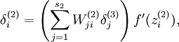
$\begin{align}J_{\rm sparse}(W,b) = J(W,b) + \beta \sum_{j=1}^{s_2} {\rm KL}(\rho || \hat\rho_j),\end{align}$

由之前的后向传递算法我们得到：

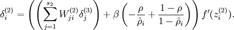
$\begin{align}\delta^{(2)}_i = \left( \sum_{j=1}^{s_{2}} W^{(2)}_{ji} \delta^{(3)}_j \right) f'(z^{(2)}_i),\end{align}$

加入稀疏约束后：

$\begin{align}\delta^{(2)}_i = \left( \left( \sum_{j=1}^{s_{2}} W^{(2)}_{ji} \delta^{(3)}_j \right)+ \beta \left( - \frac{\rho}{\hat\rho_i} + \frac{1-\rho}{1-\hat\rho_i} \right) \right) f'(z^{(2)}_i) .\end{align}$

参考资料：http://deeplearning.stanford.edu/wiki/index.php/UFLDL_Tutorial

%% CS294A/CS294W Programming Assignment Starter Code

%  Instructions
%  ------------
% 
%  This file contains code that helps you get started on the
%  programming assignment. You will need to complete the code in sampleIMAGES.m,
%  sparseAutoencoderCost.m and computeNumericalGradient.m. 
%  For the purpose of completing the assignment, you do not need to
%  change the code in this file. 
%
%%======================================================================
%% STEP 0: Here we provide the relevant parameters values that will
%  allow your sparse autoencoder to get good filters; you do not need to 
%  change the parameters below.
tic
visibleSize = 8*8;   % number of input units 
hiddenSize = 25;     % number of hidden units 
sparsityParam = 0.01;   % desired average activation of the hidden units.
                     % (This was denoted by the Greek alphabet rho, which looks like a lower-case "p",
		     %  in the lecture notes). 
lambda = 0.0001;     % weight decay parameter       
beta = 3;            % weight of sparsity penalty term       

%%======================================================================
%% STEP 1: Implement sampleIMAGES
%
%  After implementing sampleIMAGES, the display_network command should
%  display a random sample of 200 patches from the dataset

patches = sampleIMAGES;
display_network(patches(:,randi(size(patches,2),200,1)),8);


%  Obtain random parameters theta
theta = initializeParameters(hiddenSize, visibleSize);

%%======================================================================
%% STEP 2: Implement sparseAutoencoderCost
%
%  You can implement all of the components (squared error cost, weight decay term,
%  sparsity penalty) in the cost function at once, but it may be easier to do 
%  it step-by-step and run gradient checking (see STEP 3) after each step.  We 
%  suggest implementing the sparseAutoencoderCost function using the following steps:
%
%  (a) Implement forward propagation in your neural network, and implement the 
%      squared error term of the cost function.  Implement backpropagation to 
%      compute the derivatives.   Then (using lambda=beta=0), run Gradient Checking 
%      to verify that the calculations corresponding to the squared error cost 
%      term are correct.
%
%  (b) Add in the weight decay term (in both the cost function and the derivative
%      calculations), then re-run Gradient Checking to verify correctness. 
%
%  (c) Add in the sparsity penalty term, then re-run Gradient Checking to 
%      verify correctness.
%
%  Feel free to change the training settings when debugging your
%  code.  (For example, reducing the training set size or 
%  number of hidden units may make your code run faster; and setting beta 
%  and/or lambda to zero may be helpful for debugging.)  However, in your 
%  final submission of the visualized weights, please use parameters we 
%  gave in Step 0 above.

[cost, grad] = sparseAutoencoderCost(theta, visibleSize, hiddenSize, lambda, ...
                                     sparsityParam, beta, patches);

%%======================================================================
%% STEP 3: Gradient Checking
%
% Hint: If you are debugging your code, performing gradient checking on smaller models 
% and smaller training sets (e.g., using only 10 training examples and 1-2 hidden 
% units) may speed things up.

% First, lets make sure your numerical gradient computation is correct for a
% simple function.  After you have implemented computeNumericalGradient.m,
% run the following: 
checkNumericalGradient();

% Now we can use it to check your cost function and derivative calculations
% for the sparse autoencoder.  
numgrad = computeNumericalGradient( @(x) sparseAutoencoderCost(x, visibleSize, ...
                                                  hiddenSize, lambda, ...
                                                  sparsityParam, beta, ...
                                                  patches), theta);

% Use this to visually compare the gradients side by side
disp([numgrad grad]); 

% Compare numerically computed gradients with the ones obtained from backpropagation
diff = norm(numgrad-grad)/norm(numgrad+grad);
disp(diff); % Should be small. In our implementation, these values are
            % usually less than 1e-9.

            % When you got this working, Congratulations!!! 

%%======================================================================
%% STEP 4: After verifying that your implementation of
%  sparseAutoencoderCost is correct, You can start training your sparse
%  autoencoder with minFunc (L-BFGS).

%  Randomly initialize the parameters
theta = initializeParameters(hiddenSize, visibleSize);

%  Use minFunc to minimize the function
addpath minFunc/
options.Method = 'lbfgs'; % Here, we use L-BFGS to optimize our cost
                          % function. Generally, for minFunc to work, you
                          % need a function pointer with two outputs: the
                          % function value and the gradient. In our problem,
                          % sparseAutoencoderCost.m satisfies this.
options.maxIter = 400;	  % Maximum number of iterations of L-BFGS to run 
options.display = 'on';


[opttheta, cost] = minFunc( @(p) sparseAutoencoderCost(p, ...
                                   visibleSize, hiddenSize, ...
                                   lambda, sparsityParam, ...
                                   beta, patches), ...
                              theta, options);

%%======================================================================
%% STEP 5: Visualization 

W1 = reshape(opttheta(1:hiddenSize*visibleSize), hiddenSize, visibleSize);
display_network(W1', 12); 

print -djpeg weights.jpg   % save the visualization to a file 
toc

function patches = sampleIMAGES()
% sampleIMAGES
% Returns 10000 patches for training

load IMAGES;    % load images from disk 

patchsize = 8;  % we'll use 8x8 patches 
numpatches = 10000;

% Initialize patches with zeros.  Your code will fill in this matrix--one
% column per patch, 10000 columns. 
patches = zeros(patchsize*patchsize, numpatches);

%% ---------- YOUR CODE HERE --------------------------------------
%  Instructions: Fill in the variable called "patches" using data 
%  from IMAGES.  
%  
%  IMAGES is a 3D array containing 10 images
%  For instance, IMAGES(:,:,6) is a 512x512 array containing the 6th image,
%  and you can type "imagesc(IMAGES(:,:,6)), colormap gray;" to visualize
%  it. (The contrast on these images look a bit off because they have
%  been preprocessed using using "whitening."  See the lecture notes for
%  more details.) As a second example, IMAGES(21:30,21:30,1) is an image
%  patch corresponding to the pixels in the block (21,21) to (30,30) of
%  Image 1
image_N=size(IMAGES,3);
 for imageNum=1:image_N
     [row col]=size(IMAGES(:,:,imageNum));
     for PatchNum=1:numpatches
         xPix=randi([1 row-patchsize+1]);
         yPix=randi([1 col-patchsize+1]);
         patches(:,(imageNum-1)*numpatches+numpatches) = reshape( IMAGES(xPix:xPix+7,yPix:yPix+7,...
                                                                   imageNum),patchsize*patchsize,1);
     end
 end

%% ---------------------------------------------------------------
% For the autoencoder to work well we need to normalize the data
% Specifically, since the output of the network is bounded between [0,1]
% (due to the sigmoid activation function), we have to make sure 
% the range of pixel values is also bounded between [0,1]
patches = normalizeData(patches);




end


%% ---------------------------------------------------------------
function patches = normalizeData(patches)

% Squash data to [0.1, 0.9] since we use sigmoid as the activation
% function in the output layer

% Remove DC (mean of images). 
patches = bsxfun(@minus, patches, mean(patches));

% Truncate to +/-3 standard deviations and scale to -1 to 1
pstd = 3 * std(patches(:));
patches = max(min(patches, pstd), -pstd) / pstd;

% Rescale from [-1,1] to [0.1,0.9]
patches = (patches + 1) * 0.4 + 0.1;

end

function [cost,grad] = sparseAutoencoderCost(theta, visibleSize, hiddenSize, ...
                                             lambda, sparsityParam, beta, data)

% visibleSize: the number of input units (probably 64) 
% hiddenSize: the number of hidden units (probably 25) 
% lambda: weight decay parameter
% sparsityParam: The desired average activation for the hidden units (denoted in the lecture
%                           notes by the greek alphabet rho, which looks like a lower-case "p").
% beta: weight of sparsity penalty term
% data: Our 64x10000 matrix containing the training data.  So, data(:,i) is the i-th training example. 
  
% The input theta is a vector (because minFunc expects the parameters to be a vector). 
% We first convert theta to the (W1, W2, b1, b2) matrix/vector format, so that this 
% follows the notation convention of the lecture notes. 

W1 = reshape(theta(1:hiddenSize*visibleSize), hiddenSize, visibleSize);
W2 = reshape(theta(hiddenSize*visibleSize+1:2*hiddenSize*visibleSize), visibleSize, hiddenSize);
b1 = theta(2*hiddenSize*visibleSize+1:2*hiddenSize*visibleSize+hiddenSize);
b2 = theta(2*hiddenSize*visibleSize+hiddenSize+1:end);

% Cost and gradient variables (your code needs to compute these values). 
% Here, we initialize them to zeros. 
W1grad = zeros(size(W1)); 
W2grad = zeros(size(W2));
b1grad = zeros(size(b1)); 
b2grad = zeros(size(b2));

%% ---------- YOUR CODE HERE --------------------------------------
%  Instructions: Compute the cost/optimization objective J_sparse(W,b) for the Sparse Autoencoder,
%                and the corresponding gradients W1grad, W2grad, b1grad, b2grad.
%
% W1grad, W2grad, b1grad and b2grad should be computed using backpropagation.
% Note that W1grad has the same dimensions as W1, b1grad has the same dimensions
% as b1, etc.  Your code should set W1grad to be the partial derivative of J_sparse(W,b) with
% respect to W1.  I.e., W1grad(i,j) should be the partial derivative of J_sparse(W,b) 
% with respect to the input parameter W1(i,j).  Thus, W1grad should be equal to the term 
% [(1/m) \Delta W^{(1)} + \lambda W^{(1)}] in the last block of pseudo-code in Section 2.2 
% of the lecture notes (and similarly for W2grad, b1grad, b2grad).
% 
% Stated differently, if we were using batch gradient descent to optimize the parameters,
% the gradient descent update to W1 would be W1 := W1 - alpha * W1grad, and similarly for W2, b1, b2. 
% 
% W1  [w1 w2 w3...] 
J_cost = 0;
J_weight = 0;
J_sparse = 0;
[n m] = size(data);

a1 = data;    %最初的输入项
z2 = W1*data+repmat(b1,1,m); %z2 num个列  隐层单元的输入值
a2 = sigmoid(z2);  %隐层
z3 = W2*a2+repmat(b2,1,m);  %输出层的输入值
a3 = sigmoid(z3);  %输出层

%输入值和最终输出值误差
J_cost = (0.5/m)*sum(sum((a3-a1).^2));
%权值惩罚项
J_weight = 0.5*(sum(sum(W1.^2))+sum(sum(W2.^2)));
%稀疏性约束
rho = (1/m).*sum(a2,2);%隐层的平均值
J_sparse = sum( sparsityParam.*log(sparsityParam./rho) + (1-sparsityParam).*log(1-sparsityParam)./(1-rho) );

%损失函数
cost = J_cost + lambda*J_weight + beta*J_sparse;

%BP算法
d3 = -( data-a3).* sigmoidInv(z3);%输出层的误差项
sparse_term = beta*(-sparsityParam./rho) + (1-sparsityParam)./(1-rho);
d2 = (W2'*d3+repmat(sparse_term,1,m)).*sigmoidInv(z2); %隐层的误差项

W1grad = W1grad+d2*data';
W1grad = (1/m)*W1grad+lambda*W1;

W2grad = W2grad+d3*a2';
W2gard = (1/m)*W2grad + lambda*W2;

b1grad = b1grad+sum(d2,2);
b1grad = (1/m)*b1grad;

b2grad = b2grad+sum(d3,2);
b2grad = (1/m)*b2grad;

    function sig = sigmoid(x)
         sig = 1./(1+exp(-x));
    end
    function sigInv =sigmoidInv(x)
        sigInv = sigmoid(x).*(1-sigmoid(x));
    end


%-------------------------------------------------------------------
% After computing the cost and gradient, we will convert the gradients back
% to a vector format (suitable for minFunc).  Specifically, we will unroll
% your gradient matrices into a vector.

grad = [W1grad(:) ; W2grad(:) ; b1grad(:) ; b2grad(:)];

end

%-------------------------------------------------------------------
% Here's an implementation of the sigmoid function, which you may find useful
% in your computation of the costs and the gradients.  This inputs a (row or
% column) vector (say (z1, z2, z3)) and returns (f(z1), f(z2), f(z3)). 

function sigm = sigmoid(x)
  
    sigm = 1 ./ (1 + exp(-x));
end

function numgrad = computeNumericalGradient(J, theta)
% numgrad = computeNumericalGradient(J, theta)
% theta: a vector of parameters
% J: a function that outputs a real-number. Calling y = J(theta) will return the
% function value at theta. 
  
% Initialize numgrad with zeros
numgrad = zeros(size(theta));

%% ---------- YOUR CODE HERE --------------------------------------
% Instructions: 
% Implement numerical gradient checking, and return the result in numgrad.  
% (See Section 2.3 of the lecture notes.)
% You should write code so that numgrad(i) is (the numerical approximation to) the 
% partial derivative of J with respect to the i-th input argument, evaluated at theta.  
% I.e., numgrad(i) should be the (approximately) the partial derivative of J with 
% respect to theta(i).
%                
% Hint: You will probably want to compute the elements of numgrad one at a time. 


n = size(theta,1);
E = eye(n);
epsilon = 1e-4;
for i=1:n
    dtheta = E(:,i)*epsilon;
    numgrad(i) = (J(theta+dtheta)-J(theta-dtheta))/(epsilon*2.0);
end
% 
% n=size(theta,1);
% E=eye(n);
% epsilon=1e-4;
% for i=1:n
%     dtheta=E(:,i)*epsilon;
%     numgrad(i)=(J(theta+dtheta)-J(theta-dtheta))/epsilon/2.0;
% end

%% ---------------------------------------------------------------
end

function [] = checkNumericalGradient()
% This code can be used to check your numerical gradient implementation 
% in computeNumericalGradient.m
% It analytically evaluates the gradient of a very simple function called
% simpleQuadraticFunction (see below) and compares the result with your numerical
% solution. Your numerical gradient implementation is incorrect if
% your numerical solution deviates too much from the analytical solution.
  
% Evaluate the function and gradient at x = [4; 10]; (Here, x is a 2d vector.)
x = [4; 10];
[value, grad] = simpleQuadraticFunction(x);

% Use your code to numerically compute the gradient of simpleQuadraticFunction at x.
% (The notation "@simpleQuadraticFunction" denotes a pointer to a function.)
numgrad = computeNumericalGradient(@simpleQuadraticFunction, x);

% Visually examine the two gradient computations.  The two columns
% you get should be very similar. 
disp([numgrad grad]);
fprintf('The above two columns you get should be very similar.\n(Left-Your Numerical Gradient, Right-Analytical Gradient)\n\n');

% Evaluate the norm of the difference between two solutions.  
% If you have a correct implementation, and assuming you used EPSILON = 0.0001 
% in computeNumericalGradient.m, then diff below should be 2.1452e-12 
diff = norm(numgrad-grad)/norm(numgrad+grad);
disp(diff); 
fprintf('Norm of the difference between numerical and analytical gradient (should be < 1e-9)\n\n');
end


  
function [value,grad] = simpleQuadraticFunction(x)
% this function accepts a 2D vector as input. 
% Its outputs are:
%   value: h(x1, x2) = x1^2 + 3*x1*x2
%   grad: A 2x1 vector that gives the partial derivatives of h with respect to x1 and x2 
% Note that when we pass @simpleQuadraticFunction(x) to computeNumericalGradients, we're assuming
% that computeNumericalGradients will use only the first returned value of this function.

value = x(1)^2 + 3*x(1)*x(2);

grad = zeros(2, 1);
grad(1)  = 2*x(1) + 3*x(2);
grad(2)  = 3*x(1);

end

function [h, array] = display_network(A, opt_normalize, opt_graycolor, cols, opt_colmajor)
% This function visualizes filters in matrix A. Each column of A is a
% filter. We will reshape each column into a square image and visualizes
% on each cell of the visualization panel. 
% All other parameters are optional, usually you do not need to worry
% about it.
% opt_normalize: whether we need to normalize the filter so that all of
% them can have similar contrast. Default value is true.
% opt_graycolor: whether we use gray as the heat map. Default is true.
% cols: how many columns are there in the display. Default value is the
% squareroot of the number of columns in A.
% opt_colmajor: you can switch convention to row major for A. In that
% case, each row of A is a filter. Default value is false.
warning off all

if ~exist('opt_normalize', 'var') || isempty(opt_normalize)
    opt_normalize= true;
end

if ~exist('opt_graycolor', 'var') || isempty(opt_graycolor)
    opt_graycolor= true;
end

if ~exist('opt_colmajor', 'var') || isempty(opt_colmajor)
    opt_colmajor = false;
end

% rescale
A = A - mean(A(:));

if opt_graycolor, colormap(gray); end

% compute rows, cols
[L M]=size(A);
sz=sqrt(L);
buf=1;
if ~exist('cols', 'var')  %没有给定列数的情况下
    if floor(sqrt(M))^2 ~= M   %M不是平方数
        n=ceil(sqrt(M));
        while mod(M, n)~=0 && n<1.2*sqrt(M), n=n+1; end
        m=ceil(M/n);  
    else
        n=sqrt(M);
        m=n;
    end
else
    n = cols;
    m = ceil(M/n);
end

array=-ones(buf+m*(sz+buf),buf+n*(sz+buf));

if ~opt_graycolor
    array = 0.1.* array;
end


if ~opt_colmajor
    k=1;
    for i=1:m
        for j=1:n
            if k>M, 
                continue; 
            end
            clim=max(abs(A(:,k)));
            if opt_normalize
                array(buf+(i-1)*(sz+buf)+(1:sz),buf+(j-1)*(sz+buf)+(1:sz))=reshape(A(:,k),sz,sz)/clim;
            else
                array(buf+(i-1)*(sz+buf)+(1:sz),buf+(j-1)*(sz+buf)+(1:sz))=reshape(A(:,k),sz,sz)/max(abs(A(:)));
            end
            k=k+1;
        end
    end
else
    k=1;
    for j=1:n
        for i=1:m
            if k>M, 
                continue; 
            end
            clim=max(abs(A(:,k)));
            if opt_normalize
                array(buf+(i-1)*(sz+buf)+(1:sz),buf+(j-1)*(sz+buf)+(1:sz))=reshape(A(:,k),sz,sz)/clim;
            else
                array(buf+(i-1)*(sz+buf)+(1:sz),buf+(j-1)*(sz+buf)+(1:sz))=reshape(A(:,k),sz,sz);
            end
            k=k+1;
        end
    end
end

if opt_graycolor
    h=imagesc(array,'EraseMode','none',[-1 1]);
else
    h=imagesc(array,'EraseMode','none',[-1 1]);
end
axis image off

drawnow;

warning on all

转载于:https://www.cnblogs.com/learnordie/p/4656966.html

dengxundong1074

关注

0
点赞
踩
3

收藏

觉得还不错? 一键收藏
0
评论
深度学习基础（三）（稀疏）自编码器分类：深度学习 ...

我们知道在神经网络上通过前向传导和后向传导算法，可以再给定训练集的基础上训练参数，这是神经网络有监督学习的一种应用。但是有时候数据集并不是都有标签的，我们希望给一堆数据之后，通过神经网络，在没有既定目标函数的情况下，在一定约束下神经网络能够自行独立地学习到一些参数。这种没有特定学习目标的学习方法，就叫做无监督的学习方法。现在来看一种最简单的无监督神经网络算法，自编码器。自...
复制链接

扫一扫