线性分类的Jupyter实践

一、鸢尾花数据集的线性多分类

import numpy as np
from sklearn.linear_model import LogisticRegression
import matplotlib.pyplot as plt
import matplotlib as mpl
from sklearn import preprocessing
import pandas as pd
from sklearn.preprocessing import StandardScaler
from sklearn.pipeline import Pipeline

df = pd.read_csv('http://archive.ics.uci.edu/ml/machine-learning-databases/iris/iris.data', header=0)
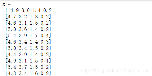
x = df.values[:, :-1]
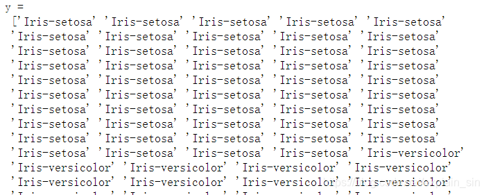
y = df.values[:, -1]
print('x = \n', x)
print('y = \n', y)
le = preprocessing.LabelEncoder()
le.fit(['Iris-setosa', 'Iris-versicolor', 'Iris-virginica'])
print(le.classes_)
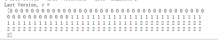
y = le.transform(y)
print('Last Version, y = \n', y)

以上为线性多分类的Python代码，需要调用numpy库、用爬虫获取鸢尾花数据集的csv文件，以及对鸢尾花的数值指标进行分类，将其分为setosa、versicolor和virginica三种不同的类型
并且在最后，此代码还有一个计数功能，分别统计三种鸢尾花的数量，输出结果如下

二、可视化显示

N, M = 500, 500     # 横纵各采样多少个值
x1_min, x1_max = x[:, 0].min(), x[:, 0].max()   # 第0列的范围
x2_min, x2_max = x[:, 1].min(), x[:, 1].max()   # 第1列的范围
t1 = np.linspace(x1_min, x1_max, N)
t2 = np.linspace(x2_min, x2_max, M)
x1, x2 = np.meshgrid(t1, t2)                    # 生成网格采样点
x_test = np.stack((x1.flat, x2.flat), axis=1)   # 测试点

cm_light = mpl.colors.ListedColormap(['#77E0A0', '#FF8080', '#A0A0FF'])
cm_dark = mpl.colors.ListedColormap(['g', 'r', 'b'])
y_hat = lr.predict(x_test)       # 预测值
y_hat = y_hat.reshape(x1.shape)                 # 使之与输入的形状相同
plt.pcolormesh(x1, x2, y_hat, cmap=cm_light)     # 预测值的显示
plt.scatter(x[:, 0], x[:, 1], c=y.ravel(), edgecolors='k', s=50, cmap=cm_dark)    
plt.xlabel('petal length')
plt.ylabel('petal width')
plt.xlim(x1_min, x1_max)
plt.ylim(x2_min, x2_max)
plt.grid()
plt.savefig('2.png')
plt.show()

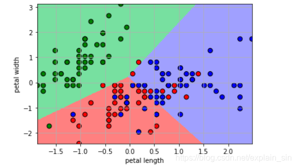
此代码主要功能为将分好类的三种鸢尾花放入长宽数值指标的坐标图中，并且进行一定量的区分，可以看到代表着红蓝两色的鸢尾花在分布方面出现了很多交叉情况，说明这两种类型拟态程度较高或者此两类区分标准不够恰当

三、精度测试实验

y_hat = lr.predict(x)
y = y.reshape(-1)
result = y_hat == y
print(y_hat)
print(result)
acc = np.mean(result)
print('准确度: %.2f%%' % (100 * acc))

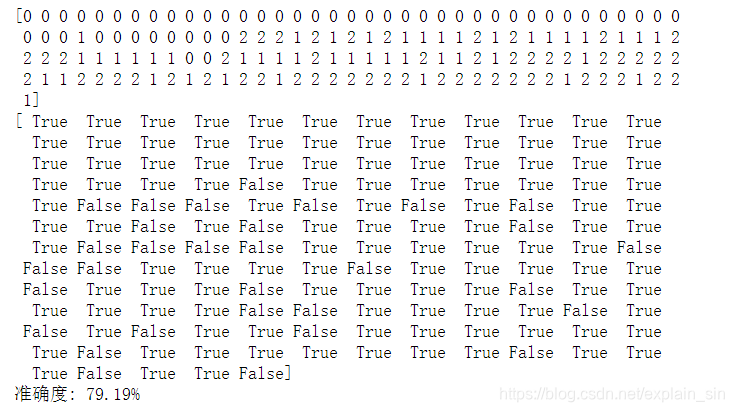
对于精度测试的代码，主要思路即为平滑输出的类型代号排序方式，比如在上列数组中第二行第四个元素是孤立的1，由排序规律可知此处应为0，所以在下表中记为False，反之则为True，最后统计True的占比即可，当然这样的精度计算存在一定误差，那就是类型交界处的代号正误难以区分，所以这里只能得出此回归方程的准确度大致为79.19％

四、参考引用

https://www.cnblogs.com/cmt/p/14553189.html
此博客链接当前不可用，或许可以在网络搜索《鸢尾花线性多分类练习.ipynb》，将此文件导入jupyter即可