Lec2.2 Regularization

Classical Regularization: Parameter Norm Penalty

54:00

Most classical regularization approaches are based on limiting the capacity of models, by adding a parameter norm penalty $\Omega (\theta )$ to the Objective function $J$.

$$J(\theta ;X,y)=J(\theta ;X,y)+\alpha \Omega (\theta )$$

$L^2$ Parameter Regularization, weight decay

Regularization term $\Omega (\theta )=\frac{1}{2}{\Vert w\Vert }_2^2$

Gradient of the total objective function:

$$\begin{gathered} {\nabla }_w\tilde{J}(w;X,y)=\alpha w+{\nabla }_{w}J(w;X,y) \\ w:=w-ϵ(\alpha w+{\nabla }_{w}J(w;X,y)) \end{gathered}$$

插播一个公式，Taylor展开式：$f(x)=f(x_0)+f^{\prime }(x_0)(x-x_0)+f^{\prime \prime }(x_0)(x-x_0{)}^2+...$

assume $w^{\star }$ is the optimal solution of $J$, that is $\nabla J(w^{\star })=0$.

$J(w)$在$w^{\star }$的Taylor展开式为：$\hat{J}(w)=J(w^{\star })+\frac{1}{2}(w-w^{\star }{)}^{T}H(w-w^{\star })$.

substitue to pervious equation,

$${\nabla }_w\tilde{J}(w;X,y)=\alpha w+H(w-w^{\star })$$, set it to $0$.

$$\begin{gathered} \alpha w+H(w-w^{\star })==0 \\ \tilde{w}=(H+\alpha I{)}^{-1}H{w}^{\star } \end{gathered}$$
$\tilde{w}$ is new solution, that’s how my solution is going to change after weight decay.

If $\alpha \to 0,\tilde{w}\to w^{\star }$, what if $\alpha$ is not 0.

H is symmetric, so it can be decomposed by $H=Q\Lambda Q^T$, substitue to the previous equation, we get, $$\begin{gathered} \tilde{w}=(Q\Lambda Q^T+\alpha I{)}^{-1}H{w}^{\star } \\ =(Q(\Lambda +\alpha I)Q^T{)}^{-1}Q\Lambda Q^T{w}^{\star } \\ =(Q(\Lambda +\alpha I{)}^{-1}{Q}^T)Q\Lambda Q^T{w}^{\star } \\ =Q(\Lambda +\alpha I{)}^{-1}\Lambda Q^T{w}^{\star } \end{gathered}$$

中间项展开式如下图所示，也是一个对角矩阵。$Q,Q^T$都可以看作旋转矩阵，并且它们两个是向相反的方向旋转。上面的等式可以这么理解：经过weight decay后的解是将原来的解，换到不同的基上，并且在每个方向都乘上一个系数。如果${\lambda }_i>>\alpha$，系数趋近于1，反之，趋近于0。这样就会去掉一些项。

Hessian matrix of $J$,代表$J$在某些方向上的变化快慢。$H=Q\Lambda Q^T$

全集

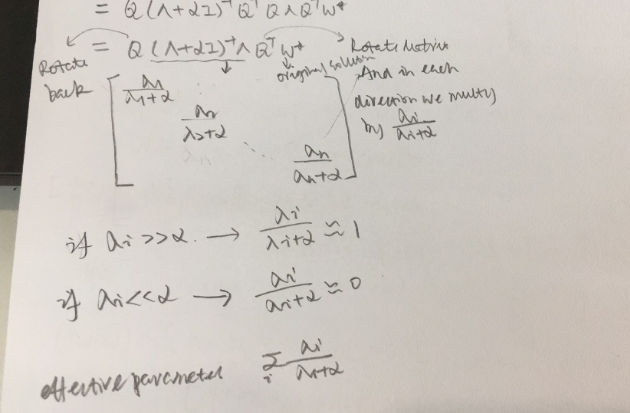
Directions along which the parameters contribute significantly to reducing the objective function are presented a small eigenvalue of the Hessian tell us that movement in this direction will not significantly increase the gradient

effective number of parameters defined to be

$$\gamma =\sum _i\frac{{\lambda }_i}{{\lambda }_i+\alpha }$$.

As $\alpha$ is increased, the effective number of parameters decreases.

Dataset Augmentation

The best way to make a machine learning model generalize better is to train it on more data.

The amount of data we have is limited.

Create fake data and add it to the training set.

Not applicable to all tasks.

For example, it is difficult to generate new fake data for a density estimation task unless we have already solved the density estimation problem.

Operations like translating the training images a few pixels in each direction can often greatly improve generalization.

One way to improve the robustness of neural networks is simply to train them with random noise applied to their inputs.

This same approach also works when the noise is applied to the hidden units, which can be seen as doing dataset augmentation at multiple levels of abstraction.

Noise injection

Two ways that noise can be used as part of a regularization strategy.

Adding noise to the input.

This can be interpreted simply as form of dataset augmentation.

Can also interpret it as being equivalent to more traditional forms of regularization.

Adding it to the weights.

This technique has been used primarily in the context of recurrent neural networks(Jim et al., 1996, Graves, 2011a).

This can be interpreted as a stochastic implementation of a Bayesian interpretation over the weights.

Manifold Tangent Classifier

It is assumed that we are trying to classify examples and that examples on the same manifold share the same category.

The classifier should be invariant to the local factors of variation that correspond to movement on the manifold.

Use an nearest-neighbor distance between points $x_1$ and $x_2$ the distance between the manifolds $M_1$ and $M_2$ to which they respectively belong.

Approximate $M_1$ by its tangent plane at $x_i$ and measure the distance between the two tangent.

Train a neural net classifier with an extra penalty to make the output $f(x)$ of the neural net locally invariant to known factors of variation(Tangent Prop algorithm, Simard et al. 1992)