14. Tensorflow2.0 梯度下降,函数优化实战,手写数字问题实战以及Tensorboard可视化！

1. 梯度下降（Gradient Descent）

1.1. What’s Gradient

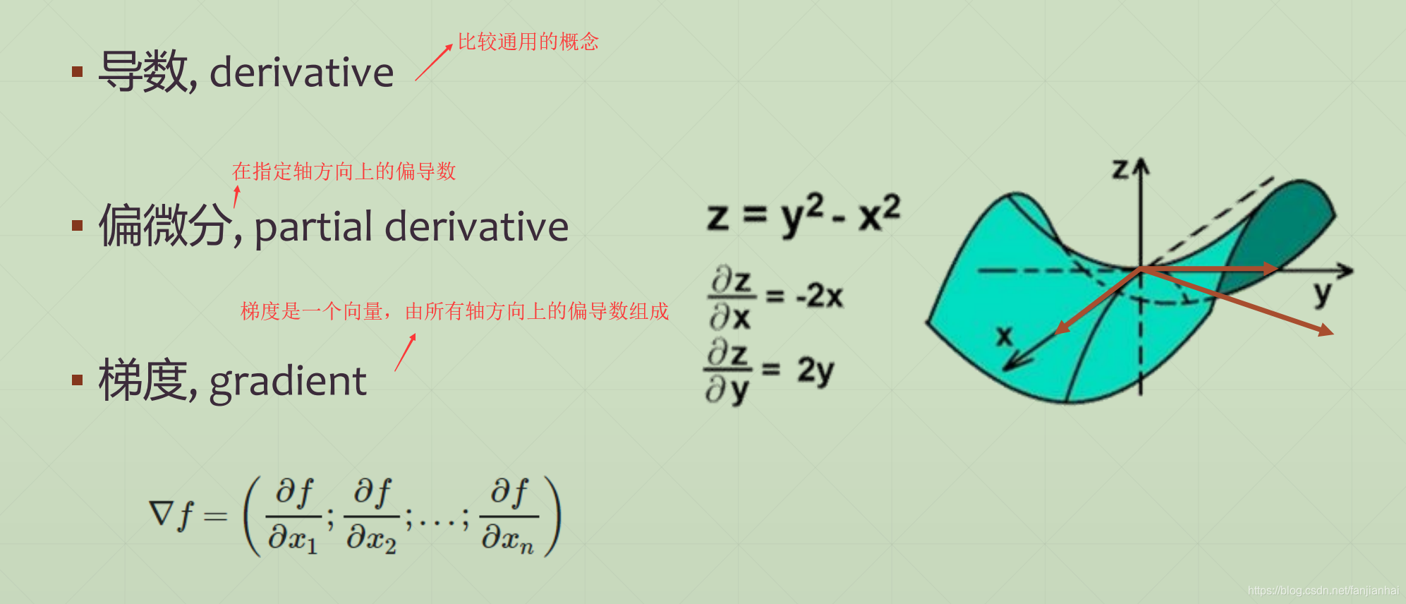
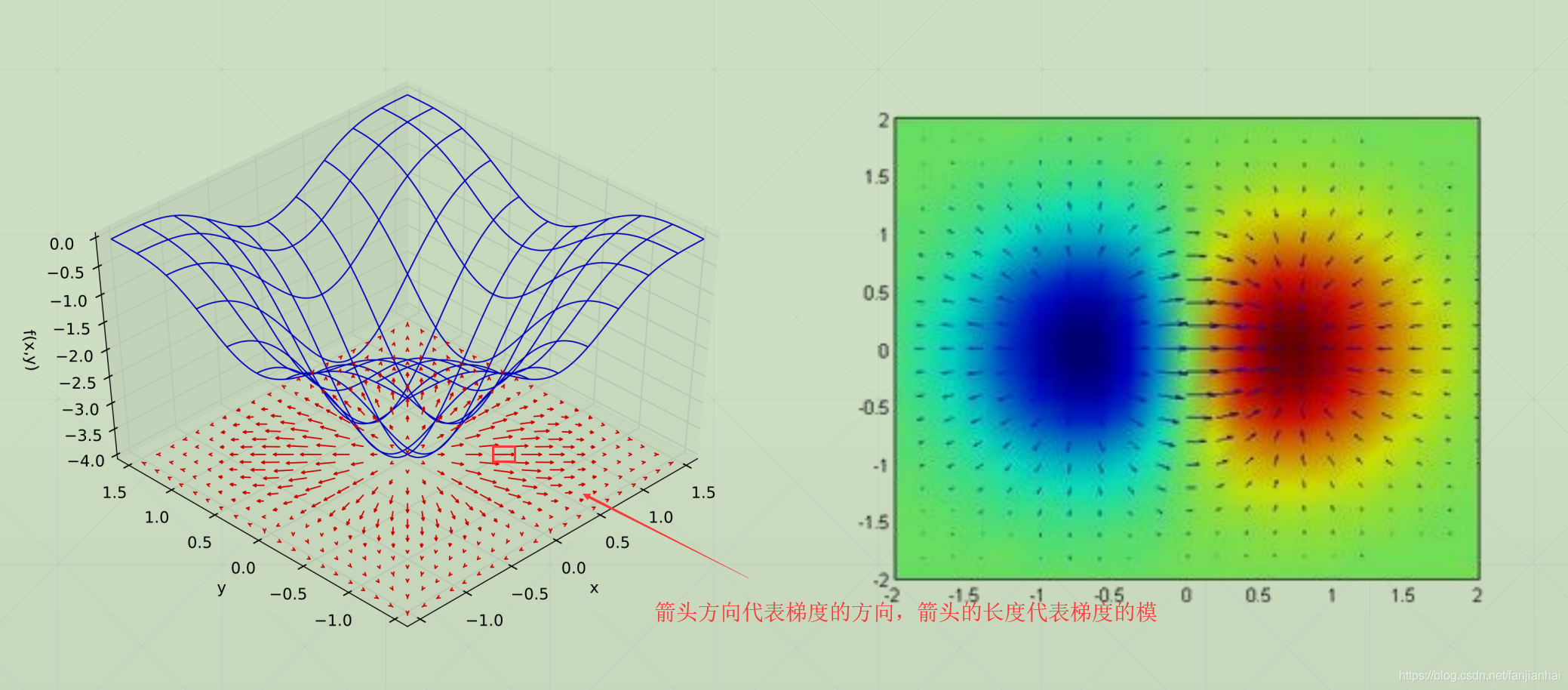
1.2. What does it mean

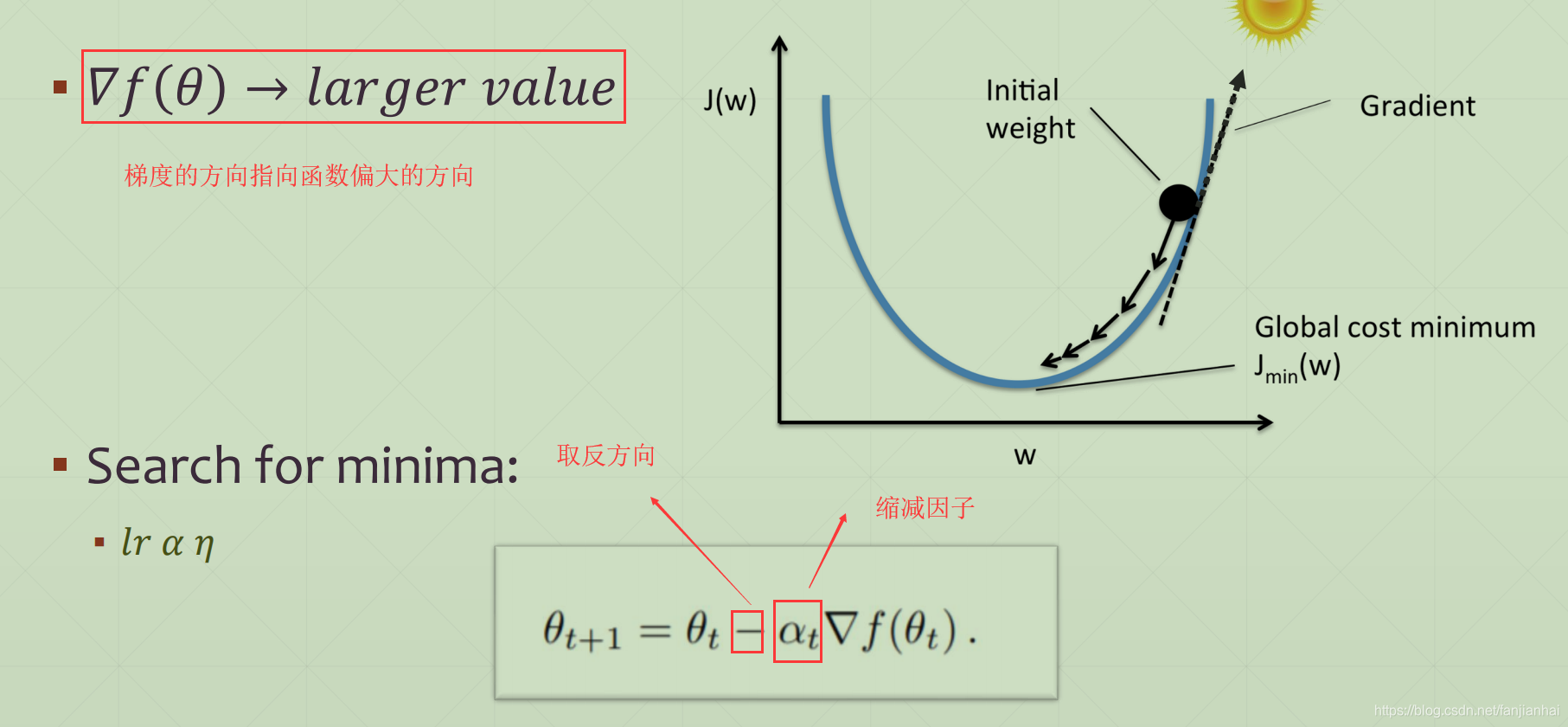
1.3. How to Search

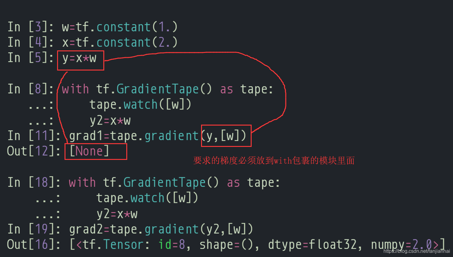
1.4. AutoGrad

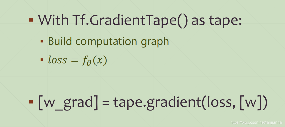
• GradientTape
  

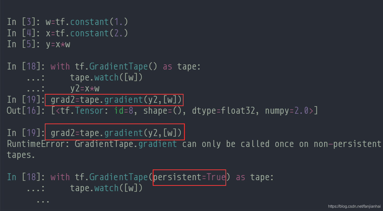
• Persistent GradientTape
  

• 2nd-order
  

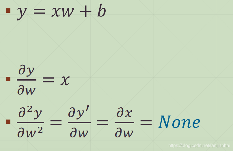
import tensorflow as tf

w = tf.Variable(1.)
b = tf.Variable(2.)
x = tf.Variable(3.)

with tf.GradientTape() as t1:
    with tf.GradientTape() as t2:
        y = x * w + b
    dy_dw, dy_db = t2.gradient(y, [w, b])
d2y_dw2 = t1.gradient(dy_dw, w)

print(dy_dw, dy_db, d2y_dw2)
assert dy_dw.numpy() == 3.0
assert d2y_dw2 is None

2. 激活函数及其梯度

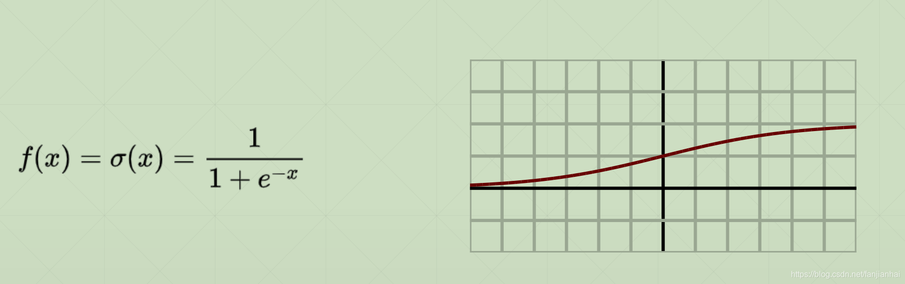
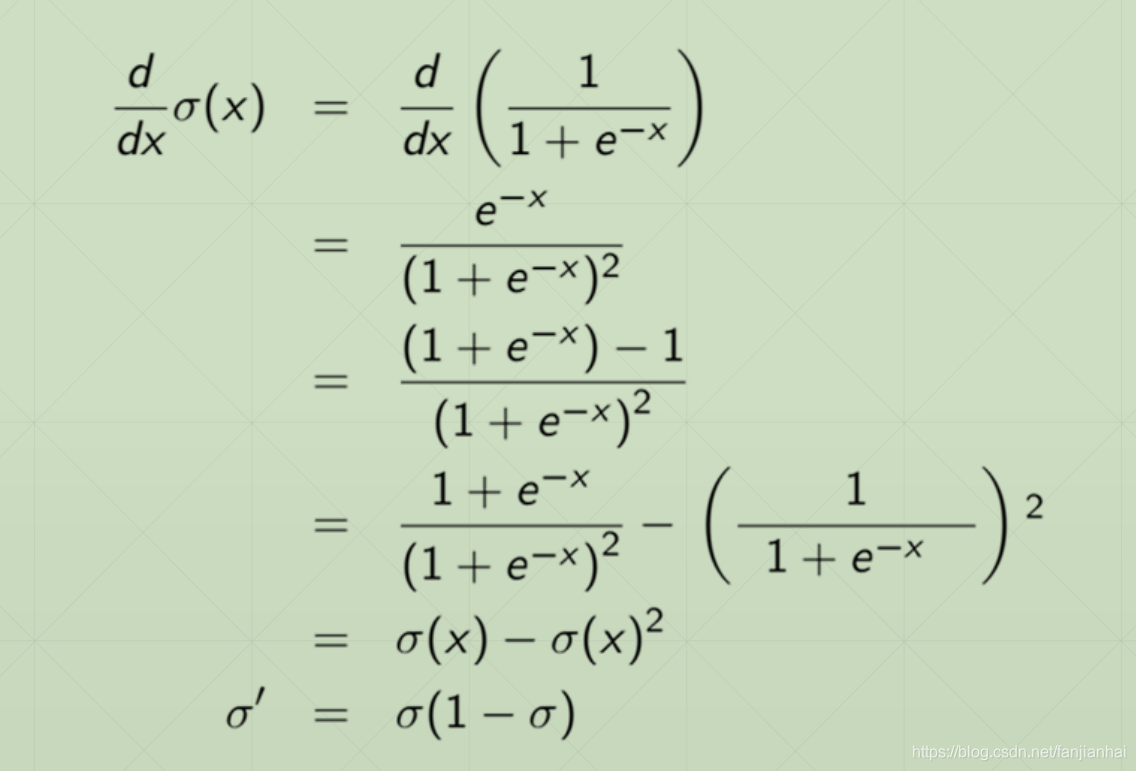
2.1. Sigmoid / Logistic（0~1）

import tensorflow as tf

a = tf.linspace(-10., 10., 10)

with tf.GradientTape() as tape:
    tape.watch(a)
    y = tf.sigmoid(a)

grads = tape.gradient(y, [a])
print(a)
print(y)
print(grads)

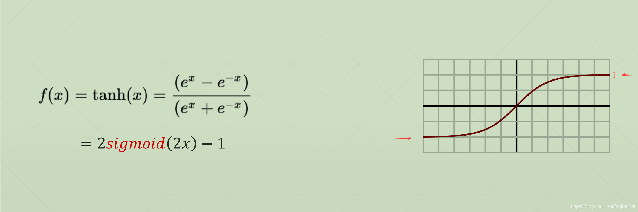
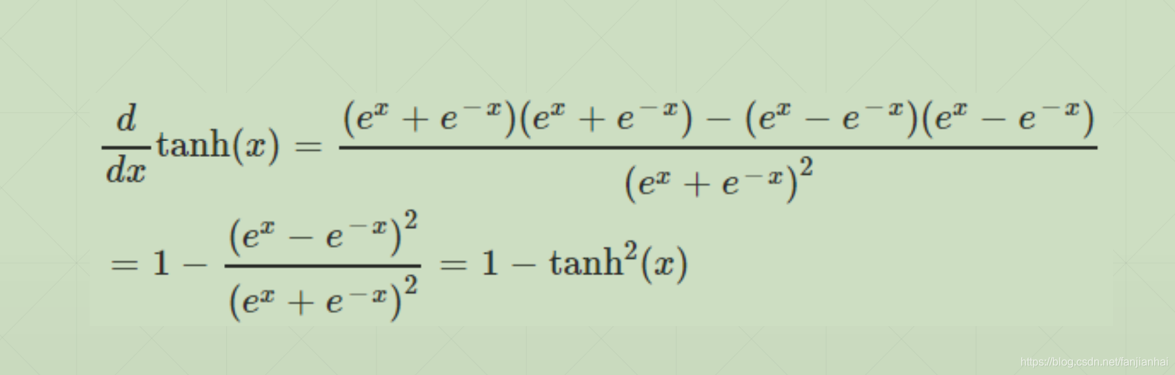
2.2. tanh（-1~1）

import tensorflow as tf

a = tf.linspace(-5., 5., 10)

with tf.GradientTape() as tape:
    tape.watch(a)
    y = tf.tanh(a)

grads = tape.gradient(y, [a])
print(a)
print(y)
print(grads)

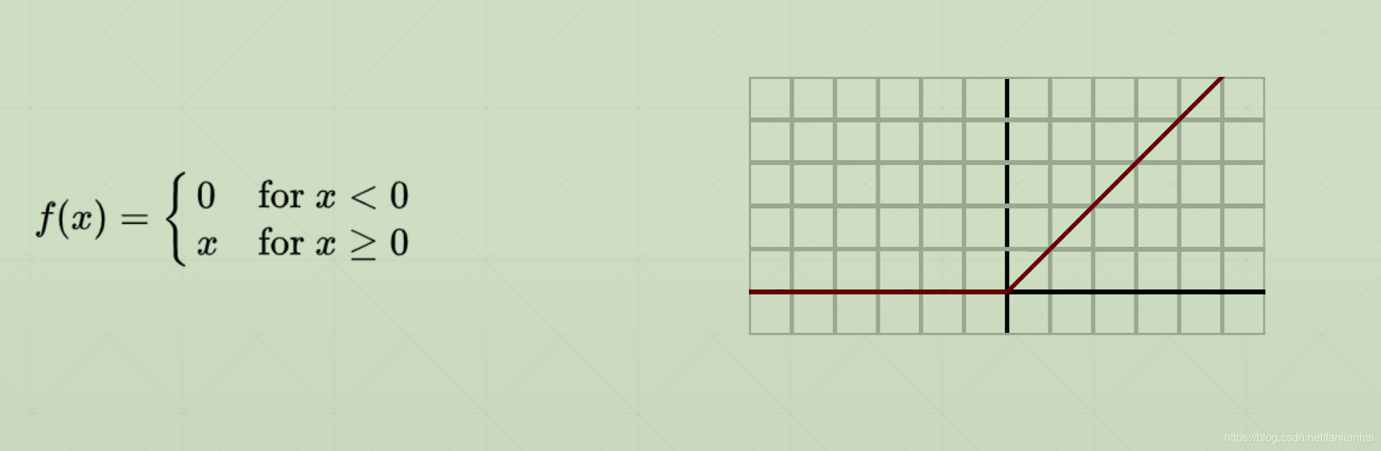
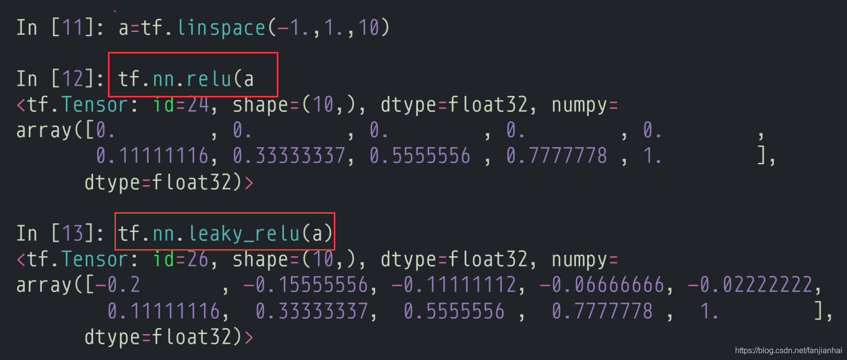
2.3. relu（Rectified Linear Unit）

3. 损失函数及其梯度

3.1. Mean Squared Error

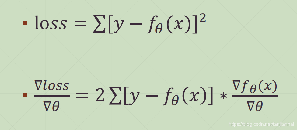
• MSE Gradient

import tensorflow as tf

x = tf.random.normal([2, 4])
w = tf.random.normal([4, 3])
b = tf.zeros([3])
y = tf.constant([2, 0])

with tf.GradientTape() as tape:
    tape.watch([w, b])  # 注意： 这里如果不写watch，则w, b必须定义成tf.Variable类型
    prob = tf.nn.softmax(x@w+b, axis=1)
    loss = tf.reduce_mean(tf.losses.MSE(tf.one_hot(y, depth=3), prob))

grads = tape.gradient(loss, [w, b])
print(grads[0])
print(grads[1])

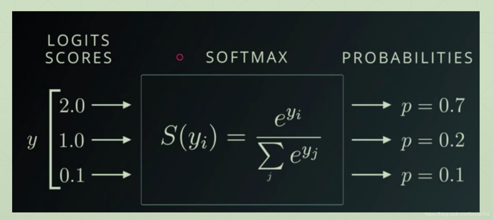
3.2. Cross Entropy Loss

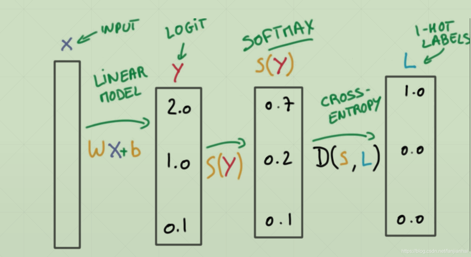
• softmax函数的作用
  • 把logit的值映射到0~1之间， 并且使得概率之后为1
  • 使强的更强，弱的更弱

• Crossentropy gradient

import tensorflow as tf

x = tf.random.normal([2, 4])
w = tf.random.normal([4, 3])
b = tf.zeros([3])
y = tf.constant([2, 0])

with tf.GradientTape() as tape:
    tape.watch([w, b])  # 注意： 这里如果不写watch，则w, b必须定义成tf.Variable类型
    logits = x@w+b
    loss = tf.reduce_mean(tf.losses.categorical_crossentropy(tf.one_hot(y, depth=3), logits, from_logits=True))

grads = tape.gradient(loss, [w, b])
print(grads[0])
print(grads[1])

4. Himmelblau函数优化

4.1. Himmelblau function

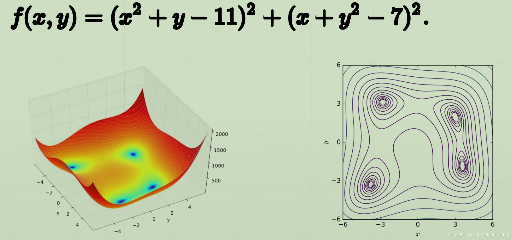
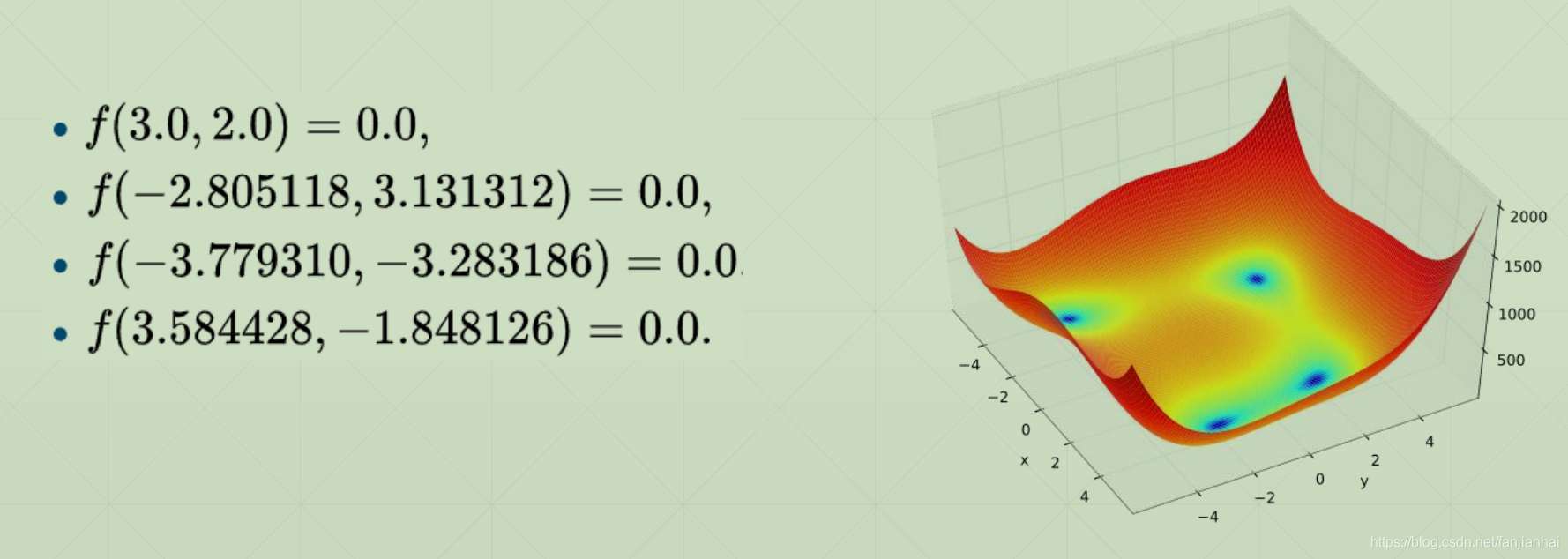
4.2. Minima

4.3. Gradient Descent

import tensorflow as tf
import numpy as np
from mpl_toolkits.mplot3d import Axes3D
from matplotlib import pyplot as plt


def himmelblau(x):
    return (x[0] ** 2 + x[1] - 11) ** 2 + (x[0] + x[1] ** 2 - 7)


x = np.arange(-6, 6, 0.1)
y = np.arange(-6, 6, 0.1)
print('x, y range:', x.shape, y.shape)
X, Y = np.meshgrid(x, y)
print('X, Y maps: ', X.shape, Y.shape)
Z = himmelblau([X, Y])

fig = plt.figure('himmelblau')
ax = fig.gca(projection='3d')
ax.plot_surface(X, Y, Z)
ax.view_init(60, -30)
ax.set_xlabel('x')
ax.set_ylabel('y')
plt.show()

# [1., 0.], [-4, 0.], [4, 0.]
x = tf.constant([-4, 0.])

for step in range(200):
    with tf.GradientTape() as tape:
        tape.watch([x])
        y = himmelblau(x)

    grads = tape.gradient(y, [x])[0]
    x -= 0.01 *grads

    if step % 20 == 0:
        print('step {}: x = {}, f(x) = {}'
              .format(step, x.numpy(), y.numpy()))

5. FashionMNIST实战

import tensorflow as tf
from tensorflow.keras import datasets, Sequential, layers, optimizers


def pre_process(x, y):
    # 在预处理之间， 数据类型已经从numpy类型转换成tensor类型
    x = tf.cast(x, dtype=tf.float32) / 255.
    y = tf.cast(y, dtype=tf.int32)
    return x, y


(x, y), (x_test, y_test) = datasets.fashion_mnist.load_data()
print(x.shape, y.shape, type(x), type(y), x.dtype, y.dtype)

db = tf.data.Dataset.from_tensor_slices((x, y))
db = db.map(pre_process).shuffle(10000).batch(128)

db_test = tf.data.Dataset.from_tensor_slices((x_test, y_test))
db_test = db_test.map(pre_process).batch(128) # 测试集不需要打散

# db_iter = iter(db)
# sample = next(db_iter)
# print("batch: ", sample[0].shape, sample[1].shape)

# 构建模型
model = Sequential([
    layers.Dense(256, activation=tf.nn.relu),  # [b, 784] ==> [b, 256]
    layers.Dense(128, activation=tf.nn.relu),  # [b, 256] ==> [b, 128]
    layers.Dense(64, activation=tf.nn.relu),   # [b, 128] ==> [b, 64]
    layers.Dense(32, activation=tf.nn.relu),   # [b, 64] ==> [b, 32]
    layers.Dense(10, activation=tf.nn.relu),   # [b, 32] ==> [b, 10]
])

model.build(input_shape=[None, 28*28])
model.summary()

# 优化器
optimizer = optimizers.Adam(learning_rate=1e-3)


def main():
    for epoch in range(30):
        for step, (x, y) in enumerate(db):
            # x: [b, 28, 28] => [b, 784]
            # y: [b]
            # 对矩阵进行变换
            x = tf.reshape(x, [-1, 28 * 28])

            with tf.GradientTape() as tape:
                # [b, 784] => [b, 10]
                logits = model(x)
                # 对真实值进行onehot编码
                y_onehot = tf.one_hot(y, depth=10)
                # 均方误差
                loss_mse = tf.reduce_mean(tf.losses.MSE(y_onehot, logits))
                # 交叉熵损失
                loss_ec = tf.reduce_mean(tf.losses.categorical_crossentropy(y_onehot, logits, from_logits=True))

            grads = tape.gradient(loss_ec, model.trainable_variables)
            optimizer.apply_gradients(zip(grads, model.trainable_variables))

            if step % 100 == 0:
                print(epoch, step, 'loss: ', float(loss_ec), float(loss_mse))

        # test
        total_correct = 0
        total_num = 0
        for x, y in db_test:
            # x:[b, 28, 28] => [b, 784]
            # y:[b]
            x = tf.reshape(x, [-1, 28*28])
            # [b, 10]
            logits = model(x)
            # logits => prob, [b, 10]
            prob = tf.nn.softmax(logits, axis=1)
            # [b, 10] => [b], int64
            pred = tf.argmax(prob, axis=1)
            pred = tf.cast(pred, dtype=tf.int32)

            correct = tf.equal(pred, y)
            correct = tf.reduce_sum(tf.cast(correct, dtype=tf.int32))
            total_correct += int(correct)
            total_num += x.shape[0]

        acc = total_correct / total_num
        print(epoch, 'test acc:', acc)


if __name__ == '__main__':
    main()
    pass

6. Tensorboard可视化

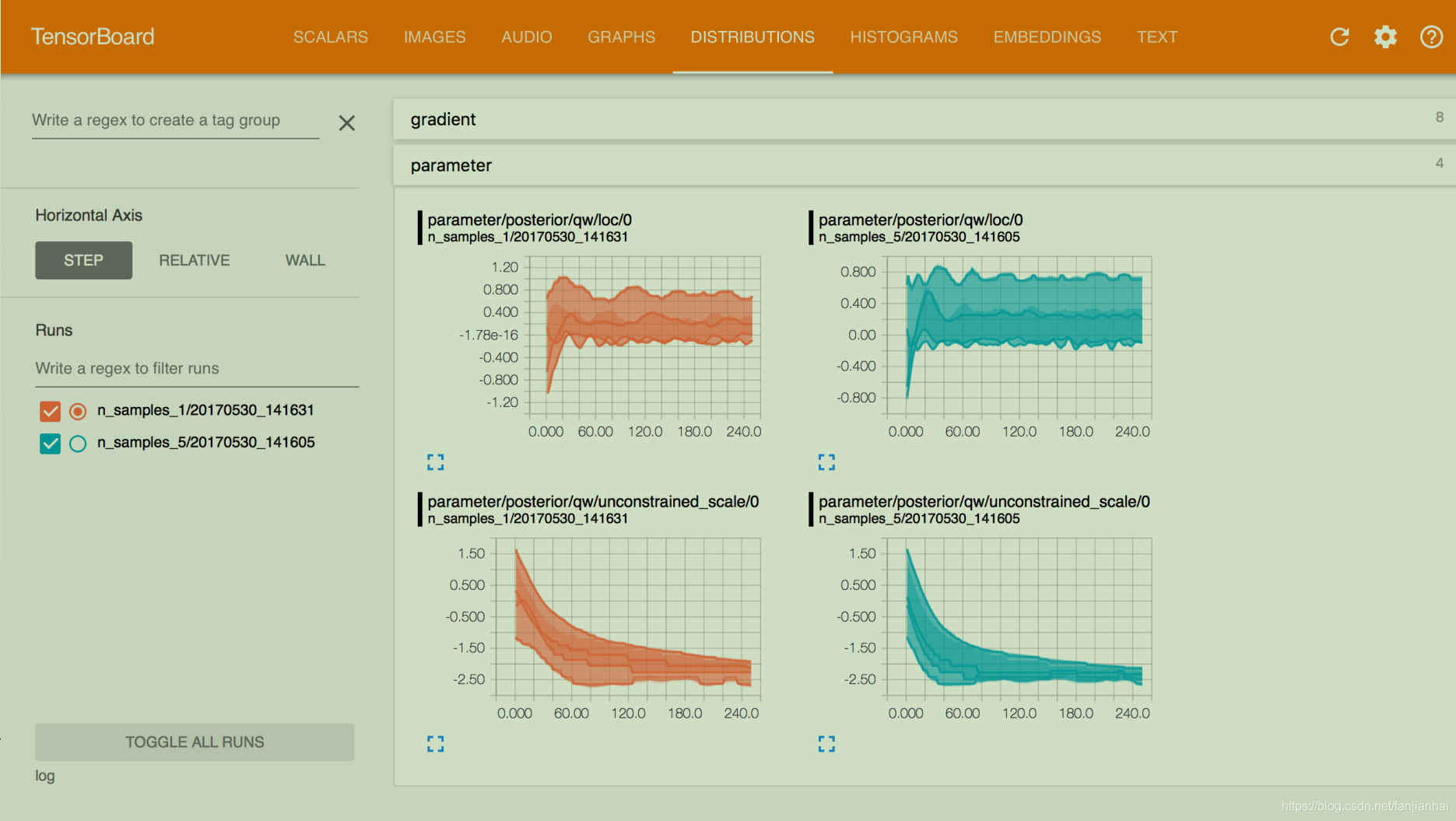
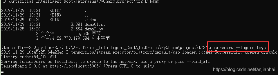
6.1. 工作原理

• Listen logdir
• build summary instance
• fed data into summary instance

6.2. Step1.run listener

6.2. Step2.build summary

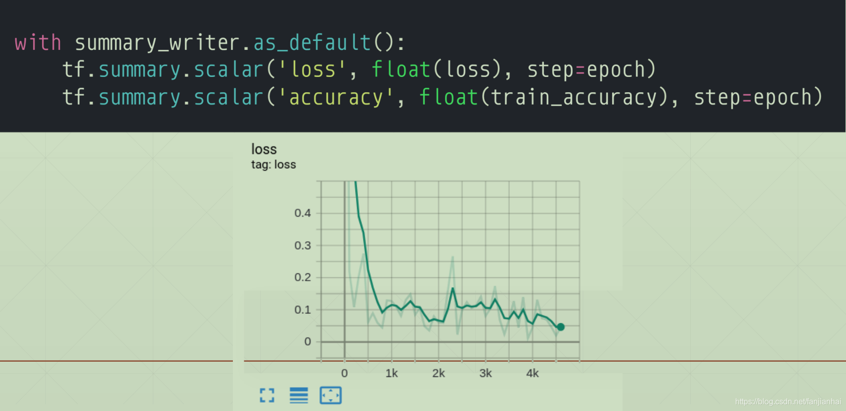
6.3. Step3.fed data

• scalar
  
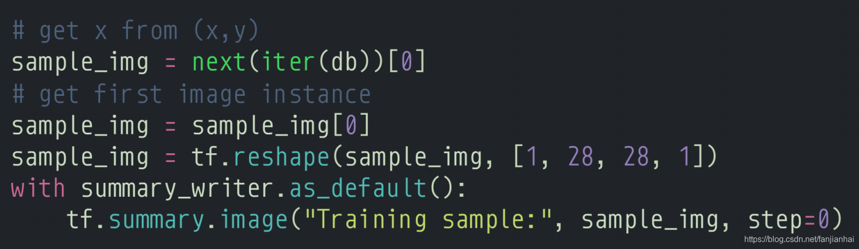
• single Image
  
  !
  
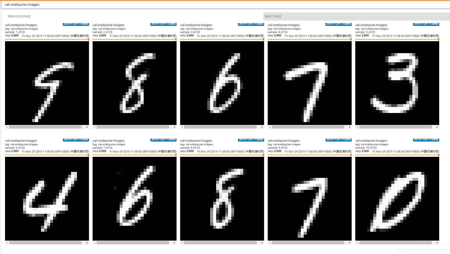
• multi image
  
  

6.4. Code

import tensorflow as tf
from tensorflow.keras import datasets, layers, optimizers, Sequential, metrics
import datetime
from matplotlib import pyplot as plt
import io


def preprocess(x, y):
    x = tf.cast(x, dtype=tf.float32) / 255.
    y = tf.cast(y, dtype=tf.int32)

    return x, y


def plot_to_image(figure):
    """Converts the matplotlib plot specified by 'figure' to a PNG image and
    returns it. The supplied figure is closed and inaccessible after this call."""
    # Save the plot to a PNG in memory.
    buf = io.BytesIO()
    plt.savefig(buf, format='png')
    # Closing the figure prevents it from being displayed directly inside
    # the notebook.
    plt.close(figure)
    buf.seek(0)
    # Convert PNG buffer to TF image
    image = tf.image.decode_png(buf.getvalue(), channels=4)
    # Add the batch dimension
    image = tf.expand_dims(image, 0)
    return image


def image_grid(images):
    """Return a 5x5 grid of the MNIST images as a matplotlib figure."""
    # Create a figure to contain the plot.
    figure = plt.figure(figsize=(10, 10))
    for i in range(25):
        # Start next subplot.
        plt.subplot(5, 5, i + 1, title='name')
        plt.xticks([])
        plt.yticks([])
        plt.grid(False)
        plt.imshow(images[i], cmap=plt.cm.binary)

    return figure


batchsz = 128
(x, y), (x_val, y_val) = datasets.mnist.load_data()
print('datasets:', x.shape, y.shape, x.min(), x.max())

db = tf.data.Dataset.from_tensor_slices((x, y))
db = db.map(preprocess).shuffle(60000).batch(batchsz).repeat(10)

ds_val = tf.data.Dataset.from_tensor_slices((x_val, y_val))
ds_val = ds_val.map(preprocess).batch(batchsz, drop_remainder=True)

network = Sequential([layers.Dense(256, activation='relu'),
                      layers.Dense(128, activation='relu'),
                      layers.Dense(64, activation='relu'),
                      layers.Dense(32, activation='relu'),
                      layers.Dense(10)])
network.build(input_shape=(None, 28 * 28))
network.summary()

optimizer = optimizers.Adam(lr=0.01)

current_time = datetime.datetime.now().strftime("%Y%m%d-%H%M%S")
log_dir = 'logs/' + current_time
summary_writer = tf.summary.create_file_writer(log_dir)

# get x from (x,y)
sample_img = next(iter(db))[0]
# get first image instance
sample_img = sample_img[0]
sample_img = tf.reshape(sample_img, [1, 28, 28, 1])
with summary_writer.as_default():
    tf.summary.image("Training sample:", sample_img, step=0)

for step, (x, y) in enumerate(db):

    with tf.GradientTape() as tape:
        # [b, 28, 28] => [b, 784]
        x = tf.reshape(x, (-1, 28 * 28))
        # [b, 784] => [b, 10]
        out = network(x)
        # [b] => [b, 10]
        y_onehot = tf.one_hot(y, depth=10)
        # [b]
        loss = tf.reduce_mean(tf.losses.categorical_crossentropy(y_onehot, out, from_logits=True))

    grads = tape.gradient(loss, network.trainable_variables)
    optimizer.apply_gradients(zip(grads, network.trainable_variables))

    if step % 100 == 0:
        print(step, 'loss:', float(loss))
        with summary_writer.as_default():
            tf.summary.scalar('train-loss', float(loss), step=step)

            # evaluate
    if step % 500 == 0:
        total, total_correct = 0., 0

        for _, (x, y) in enumerate(ds_val):
            # [b, 28, 28] => [b, 784]
            x = tf.reshape(x, (-1, 28 * 28))
            # [b, 784] => [b, 10]
            out = network(x)
            # [b, 10] => [b]
            pred = tf.argmax(out, axis=1)
            pred = tf.cast(pred, dtype=tf.int32)
            # bool type
            correct = tf.equal(pred, y)
            # bool tensor => int tensor => numpy
            total_correct += tf.reduce_sum(tf.cast(correct, dtype=tf.int32)).numpy()
            total += x.shape[0]

        print(step, 'Evaluate Acc:', total_correct / total)

        # print(x.shape)
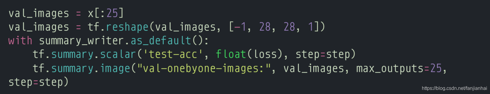
        val_images = x[:25]
        val_images = tf.reshape(val_images, [-1, 28, 28, 1])
        with summary_writer.as_default():
            tf.summary.scalar('test-acc', float(total_correct / total), step=step)
            tf.summary.image("val-onebyone-images:", val_images, max_outputs=25, step=step)

            val_images = tf.reshape(val_images, [-1, 28, 28])
            figure = image_grid(val_images)
            tf.summary.image('val-images:', plot_to_image(figure), step=step)

7. 需要全套课程视频+PPT+代码资源可以私聊我

• 方式1：CSDN私信我!
• 方式2：QQ邮箱:594042358@qq.com或者直接加我QQ: 594042358!