MATLAB神经网络编程（七）——BP神经网络的实现

《MATLAB神经网络编程》 化学工业出版社 读书笔记
第四章 前向型神经网络 4.3 BP传播网络

本文是《MATLAB神经网络编程》书籍的阅读笔记，其中涉及的源码、公式、原理都来自此书，若有不理解之处请参阅原书

---

本文讲述BP网络常用的两个例子：函数逼近与噪声消除

【例4-34】利用一个单隐层的BP网络来逼近一个函数。

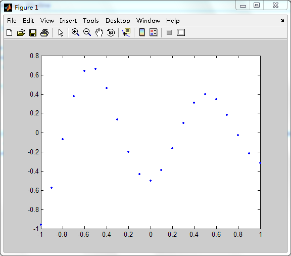
通过对函数进行采样得到了网络的输入变量P和目标变量T，在M文件中输入以下命令：

 P=-1:0.1:1;
T=[-0.9602 -0.5770 -0.0729 0.3771 0.6405 0.6600 0.4600 0.1336 -0.2013 -0.4344 -0.5000...
   -0.3930 -0.1647 0.0988 0.3072 0.3960 0.3449 0.1816 -0.0312 -0.2189 -0.3201];

每组向量都有21组数据，可以将输入向量和目标向量绘制在一起，如下图：

该网络的输入层与输出层的神经元个数均为1，根据以上的隐含层设计经验公式（时间久了，不记得这个公式在哪里了），以及考虑本例的实际情况，解决该问题的网络的隐层神经元个数应该在3~8之间。因此，下面设计一个隐含层神经元数目可变的BP网络，通过误差比，确定最佳的隐含层神经元个数，并检验隐含层神经元个数对网络性能的影响。
在M文件中输入命令：

P=-1:0.1:1;
T=[-0.9602 -0.5770 -0.0729 0.3771 0.6405 0.6600 0.4600 0.1336 -0.2013 -0.4344 -0.5000...
   -0.3930 -0.1647 0.0988 0.3072 0.3960 0.3449 0.1816 -0.0312 -0.2189 -0.3201];
s=3:8;
res=1:6
for i=1:6
    net=newff(minmax(P),[s(i),1],{'tansig','logsig'},'traingdx');
    net.trainParam.epochs=2000;
    net.trainParam.goal=0.001;
    net=train(net,P,T)
    y=sim(net,P);
    error=y-T;
    res(i)=norm(error)
end;

程序输出：

net =

    Neural Network object:

    architecture:

         numInputs: 1
         numLayers: 2
       biasConnect: [1; 1]
      inputConnect: [1; 0]
      layerConnect: [0 0; 1 0]
     outputConnect: [0 1]

        numOutputs: 1  (read-only)
    numInputDelays: 0  (read-only)
    numLayerDelays: 0  (read-only)

    subobject structures:

            inputs: {1x1 cell} of inputs
            layers: {2x1 cell} of layers
           outputs: {1x2 cell} containing 1 output
            biases: {2x1 cell} containing 2 biases
      inputWeights: {2x1 cell} containing 1 input weight
      layerWeights: {2x2 cell} containing 1 layer weight

    functions:

          adaptFcn: 'trains'
         divideFcn: (none)
       gradientFcn: 'calcgrad'
           initFcn: 'initlay'
        performFcn: 'mse'
          plotFcns: {'plotperform','plottrainstate','plotregression'}
          trainFcn: 'traingdx'

    parameters:

        adaptParam: .passes
       divideParam: (none)
     gradientParam: (none)
         initParam: (none)
      performParam: (none)
        trainParam: .show, .showWindow, .showCommandLine, .epochs, 
                    .time, .goal, .max_fail, .lr, 
                    .lr_inc, .lr_dec, .max_perf_inc, .mc, 
                    .min_grad

    weight and bias values:

                IW: {2x1 cell} containing 1 input weight matrix
                LW: {2x2 cell} containing 1 layer weight matrix
                 b: {2x1 cell} containing 2 bias vectors

    other:

              name: ''
          userdata: (user information)


res =

    1.5775    1.8000    1.9073    1.5776    1.4413    1.4408

由此可见，网络的隐含层神经元的传递函数为tansig，输出层神经元的传递函数是logsig，因为目标向量的元素都位于区间[-1,1]中，正好满足函数tansig的输出要求。
以上结果表明，在经过2000次训练后（训练函数traingdx），隐含层神经元为8的BP网络对函数的逼近效果最好，因为他的误差最小，而且网络经过27次训练就达到了目标误差。隐含层为6和9的网络误差也比较小，但是他们需要的训练时间比较长。考虑到网络性能的训练速度，这里把网络隐含层的神经元数目设定为8。
当隐含层神经元数目是8时，网络的逼近误差是1.4407.网络的训练过程记录如下：

通过对训练好的网络进行仿真，可以得到网络对函数的逼近情况，输入下面命令：

y=sim(net,P);
plot(P,T,'rp');
hold on
plot(P,y,'.');
legend('原始网络','训练后的网络');
 plot(1:21,y-T);

得到函数的逼近结果与误差曲线：

---

---

【例4-35】利用BP神经网络去除噪声问题。
在MATLAB神经网络工具箱中，提供了26个大写字母的数据矩阵，利用BP神经网络，可以进行字符识别处理。
源码：

%训练样本数据点
[AR,TS]=prprob;
A=size(AR,1);
B=size(AR,2);
C2=size(TS,1);
%测试样本数据点
CM=AR( : ,13)
noisyCharM=AR(:,13)+rand(A,1)*0.3
figure
plotchar(noisyCharM)
%创建BP网络，并使用数据点训练网络
P=AR;
T=TS;
%输入层包含10个神经元，输出层为C2(26)个神经元，输入输出层分别使用logsig传递函数
net=newff(minmax(P),[10,C2],{'logsig','logsig'},'traingdx');
net.trainParam.show=50;
net.trainParam.lr=0.1;
net.trainParam.lr_inc=1.05;
net.trainParam.epochs=3000;
net.trainParam.goal=0.01;
[net,tr]=train(net,P,T);

%回带检验
A=sim(net,CM)
%测试样本检验
a=sim(net,noisyCharM)
%找到字母所在的位置
pos=find(compet(a)==1)
figure
%绘制去除噪声后的字母
plotchar(AR(:,pos))

训练过程：

实验的结果：

可见BP网络去除了字母M上的随机噪声。

---