朴素贝叶斯的python实现（针对算法预测类不针对文本）

首先，感谢Chai_zheng博主提供的代码思路，本文代码基于该博主思路所编写！！！感谢这个开源的时代。

一、贝叶斯原理:

作为一名研究（虽然是菜鸟级别的，哈哈），那还是用学习贝叶斯的人员来自称吧，还是要吹一下贝叶斯的几大优点的。

贝叶斯网络是一种概率图形模型，广泛应用于各种人工智能推理和因果建模中。在众多的分类模型中，贝叶斯网络对处理不确定性推理有着明显的优势。它主要用概率刻画因果关系，并可以处理存在噪声信息或者数据缺失的数据集。最重要的是贝叶斯网络是一种简单的、可解释分类模型，可在多场合提供决策支持。贝叶斯网络分为结构学习和参数学习两个部分。结构学习是形成一个有向无环图（DAG）的过程，图中节点代表属性，有向边代表属性间的条件关系或因果关系。参数学习以条件概率分布刻画属性对其父节点的依赖关系，通过样本的频率表示概率并填充条件概率表。从1988年Pearl提出贝叶斯网络后，经过近三十年的发展形成了很多新算法，具有代表性的有朴素贝叶斯(Naive Bayes，NB)、树增广朴素贝叶斯模型(Tree-Augmented Naive Bayes，TAN)和K阶贝叶斯分类模型(k-dependence Bayesian Cla-ssifier，KDB)【后面的算法打算自己慢慢的用python实现，敬请期待】

进入正题，在贝叶斯理论中有一个十分重要的假设就是条件独立性假设，该假设可以描述为除了父节点外，节点Xi与其他节点无依赖关系（即相互独立），这一点是贝叶斯研究成立的树根，为了便于理解画个草图（如图1）。X5只与Y有关，X3只与X5和Y有关，与X3相互独立,但对于朴素贝叶斯来说非类节点之间相互独立（即没有弧）。

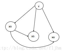
图1

贝叶斯网络能处理离散数据和连续数据，不同的平台处理这两种数据利用的原理大致相同，利用条件独立性假设，离散数据的条件概率计算公式如下：

P(Xi|Y)=P(Y)∏P(Xi|Y)

对于任意给定的随机样本集x =(x1 ,x2 ,··· ,xn ),其对应的联合概率分布表示如下:

P(c,x)
= P(c)P(x1|c)P(x2 |c)···P(xn |c)
= P(c)∏P(x i |c) (i=1...N)

其中P(c)为类先验概率.

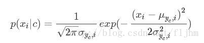
对于连续数据用概率密度函数来计算P(Xi|C)，其中μ，σ分别代表数据的均值和标准差

二、建模的基本思路

1、计算先验概率，离散的就计算条件概率，连续的就计算概率密度

2、根据训练集训练模型（朴素贝叶斯就是得到先验概率Pc，均值，标准差）

3、根据测试集测试模型，和真实标签值进行比较，预测对了就累加matchCount

4、matchCount/测试集总数据= 准确率

三，python代码如下

（代码最后自己敲一下没这样才有意义，有些地方不懂的自己打印出来看看，理解了才是重点）

好看的代码千篇一律，各自的理解万里无一。（源自：好看皮囊千篇一律，有趣的灵魂万里无一，^_^）

采用葡萄酒（wine.txt）数据集进行测试，取测试集占比0.4，在72个测试样本上正确率为95%-100%（抽取样本的随机性导致结果不同），足见其实用性的是下载地址链接: https://pan.baidu.com/s/1i4E78VF 密码: 5u8x   别人可能需要积分，这个不需要积分，百度分享，本就是uci上捐赠的数据集，【如有侵权请及时私信】

# coding=utf-8

import math
import time
import numpy as np
from collections import Counter
from sklearn import preprocessing
from sklearn.model_selection import train_test_split


def calcProbDensity(meanLabel, stdLabel, test_X):
    numAttributes = len(test_X)
    MultiProbDensity = 1.0
    print "this is calcPD"
    # print meanLabel
    # print stdLabel
    for i in range(numAttributes):
        MultiProbDensity *= np.exp(-np.square(test_X[i] - meanLabel[i]) / (2.0 * np.square(stdLabel[i]))) / (
            np.sqrt(2.0 * math.pi) * stdLabel[i])
    print MultiProbDensity
    return MultiProbDensity


def calcPriorProb(Y_train):  # 计算先验概率P(c)
    i, j = 0, 0
    global labelValue, classNum
    numSamples = Y_train.shape[0]  # 读取Y_train的第一维度的长度,比如多少行。
    labelValue = np.zeros((numSamples, 1))  # 用前i行来保存标签值
    # print "laV:",labelValue
    Y_train_counter = sum(Y_train.tolist(), [])  # 将Y_train转化为可哈希的数据结构
    cnt = Counter(Y_train_counter)  # 计算标签值的类别个数{1,2,3}及各类样例的个数
    # print "cnt",cnt
    for key in cnt:
        labelValue[i] = key
        i += 1
    classNum = i
    # print "laV2:",labelValue
    # print classNum
    Pc = np.zeros((classNum, 1))  # 不同类的先验概率
    eachLabelNum = np.zeros((classNum, 1))  # 每类样例数,多少行多少列，这里是classNum行1列
    for key in cnt:
        Pc[j] = float(cnt[key]) / numSamples #这里加float是为了避免/整除号使Pc=0
        eachLabelNum[j] = cnt[key]
        j += 1
    return labelValue, eachLabelNum, classNum, Pc


def trainBayes(X_train, Y_train):
    startTime = time.time()
    numTrainSamples, numAttributes = X_train.shape
    print "trainBayes"
    # print numAttributes,numTrainSamples
    labelValue, eachLabelNum, classNum, Pc = calcPriorProb(Y_train)
    meanlabelX, stdlabelX = [], []  # 存放每一类样本在所有属性上取值的均值和方差

    for i in range(classNum):
        k = 0
        labelXMaxtrix = np.zeros((int(eachLabelNum[i]), numAttributes))
        for j in range(numTrainSamples):
            if Y_train[j] == labelValue[i]:
                labelXMaxtrix[k] = X_train[j, :]
                k += 1
        meanlabelX.append(np.mean(labelXMaxtrix, axis=0).tolist())  # 求该矩阵的列均值与无偏标准差，append至所有类
        stdlabelX.append(np.std(labelXMaxtrix, ddof=1, axis=0).tolist())
    meanlabelX = np.array(meanlabelX).reshape(classNum, numAttributes)
    stdlabelX = np.array(stdlabelX).reshape(classNum, numAttributes)
    # print meanlabelX
    # print "###"
    # print stdlabelX
    print('---Train completed.Took %f s.' % ((time.time() - startTime)))
    return meanlabelX, stdlabelX, Pc


def predict(X_test, Y_test, meanlabelX, stdlabelX, Pc):
    numTestSamples = X_test.shape[0]
    matchCount = 0
    for m in range(X_test.shape[0]):
        x_test = X_test[m, :]  # 轮流取测试样本
        pred = np.zeros((classNum, 1))  # 对不同类的概率
        print "Pc:", Pc
        for i in range(classNum):
            pred[i] = calcProbDensity(meanlabelX[i, :], stdlabelX[i, :], x_test) * Pc[i]  # 计算属于各类的概率
            # print i
        print pred
        predict1 = labelValue[np.argmax(pred)]  # 取最大的类标签,np.argmax(pred)返回最大数据所在的index
        print predict1, "####", Y_test[m]
        if predict1 == Y_test[m]:
            matchCount += 1
        print "matchCount", matchCount, numTestSamples
    accuracy = float(matchCount) / numTestSamples #这里加float是为了避免/整除号使accuracy=0
    # print accuracy
    return accuracy


if __name__ == '__main__':
    print('Step 1.Loading data...')
    # 数据集下载http://download.csdn.net/download/chai_zheng/10009919
    data = np.loadtxt("data/wine.txt", delimiter=',')  # 载入葡萄酒数据集
    print('---Loading completed.')
    x = data[:, 1:14]
    y = data[:, 0].reshape(178, 1)
    # print x
    # print "!!!!"
    # print y
    print('Step 2.Splitting and preprocessing data...')
    X_train, X_test, Y_train, Y_test = train_test_split(x, y, test_size=0.4)  # 拆分数据集
    scaler = preprocessing.StandardScaler().fit(X_train)  # 数据标准化
    X_train = scaler.transform(X_train)
    X_test = scaler.transform(X_test)
    print('---Splittinging completed.\n---Number of training samples:%d\n---Number of testing samples:%d' \
          % (X_train.shape[0], X_test.shape[0]))
    print('Step 3.Training...')
    meanlabelX, stdlabelX, Pc = trainBayes(X_train, Y_train)
    print('Step 4.Testing...')
    accuracy = predict(X_test, Y_test, meanlabelX, stdlabelX, Pc)
    print('---Testing completed.Accuracy:%.3f%%' % (accuracy * 100))

结果截图：