Numerical solution -- Ch.1

§ 首先简化运算

1. 并行: Matlab parpool

2. 化简/减少指数运算，增加加减

e.g. Horner’s Methods (多项式）
$x^5+x^4+x^3+x^2+x$
转换为:
$x\ast (x\ast (x\ast (x\ast (x+1)+1)+1)+1)$
转化后, 计算效率高!

Matlab code

syms x
h = x^5 + x^4 + x^3 + x^2 + x;
horner(h)

test

x = randn(1000, 50);
tic;
for ii = 1:100
    A = x.^5 + x.^4 + x.^3 + x.^2 + x;
end
t1 = toc;

tic;
for ii = 1:100
    B = x.*(x.*(x.*(x.*(x + 1) + 1) + 1) + 1);
end
t2 = toc;
assert(max(max(abs(A - B))) < 1e-12);
t1/t2

§ 1. Stopping rules

p50

stopping rule 1: stop when the sequence does not change much

|Xk-Xk+1|/（1+|Xk|） < \epsilon
（take into consideration that Xk could converege to 0)
Note: This is NOT the golden rule. We need to infer some qualitative properties from the formula and use this to judge if the result is reasonable or not.

stopping rule 2: rate of convergence

§2 Evaluating error: 应对结果准确度进行评估

1. ||x*-$\hat{x}$||

Use some special cases (parameter value) to test the credibility of algorithm

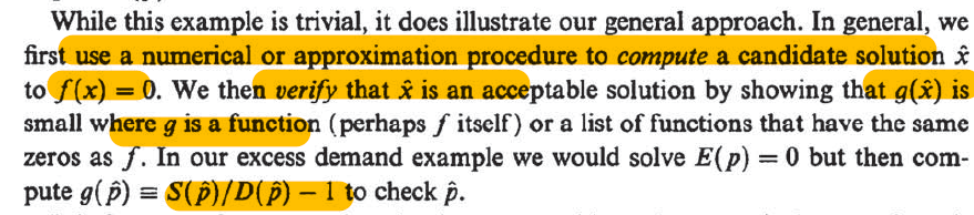
2. In many cases, the true solution x* is unknown

– Measure the extent to which the result of computation viloate properties/conditions satisfied by the true solution
– 可以比较f(x)与$f(\hat{x})$. In particular, we can rearrange f(x) s.t. f(x) = 0, then compare 0 with $f(\hat{x})$, normalized by some element

考虑误差是否可以接受，应结合目标值大小
e.g. E( p ) = D( p )-S( p )

§ 3 Computational complexity