R语言 | 单元变量的数据可视化方法

Uni-variate data  一元变量的数据分析方法

代码库在https://github.com/TigerInnovate/DataAnalysisWithR

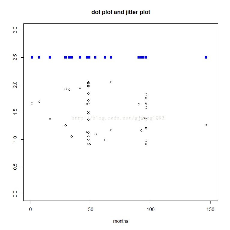
点图dot plot与抖动图jitter plot

当点都重叠在一起的时候，为了更直观分析数据分布情况，可以把点适当抖动到一定位置（适量的偏移）。

下面这个例子，由于x的值是我们要观测的，所以在y上进行抖动。不可以在x上抖动，因为x是观测对象。

一个tip：空心圆圈，是最容易识别的图形。填充的图形造成难以识别内部结构，而线（框或叉）在数据量大的时候往往难以识别。

数据文件 presidents.txt

presidents <- read.fwf("presidents.txt", widths = c(9, 15, 3), col.names = c("id","name","months"))

with(
  data=presidents, 
   {
    plot(months, rep(2.5, length(months)),
         main = "dot plot and jitter plot",
         xlab = "months", ylab = "",
         pch = 15, col = "blue", 
         xlim = c(0, 150), ylim=c(0, 3))
    
    points(months, jitter(rep(1.5, length(months)), 20), col = "black")
    })

柱状图 Histogram

柱状图用于分析单元数据的分布。

假设垂直的柱状图：每根柱子有一个宽度，待分析的数据落在柱子的宽度区间内，则进行相应的计数。y是数据落在每个宽度区间内的元素个数，决定了柱子的高度。y值可以是绝对的count，也可以是相对的百分比 binCount/N。binCount是每个柱子绝对的count，N是总的样本数量。

实验数据：serverdata.txt

决定柱状图形状有两个参数：

1. 每根柱子的宽度 bin width （分箱宽度）

bin width太宽，会丢失很多细节信息。太窄，会导致很多箱子都没有数据，从而数据分布的形状不够显而易见。

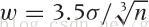
选择好的bin width很重要。对于正态分布，可以尝试使用Scott rule: 

serverdata <- read.table("serverdata.txt", col.names="CPU")
with(
  data=serverdata,

  {
    w=trunc((3.5*sd(CPU)) / (length(CPU)^(1/3)))
    par(mfrow=c(2,1))
    hist(CPU,breaks=w,freq=T, main = "frequency histogram")
    hist(CPU,breaks=w,freq=F, main = "Non frequency histogram")
  }
)

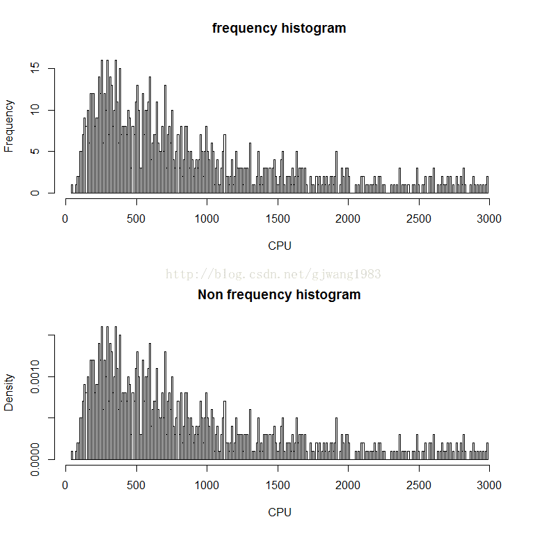
bin witdth可以不一样宽：

注意 breaks是一个递增向量，箱宽由当前减去前一个所得。

> op <- par(mfrow = c(2, 2))
> hist(islands)
> utils::str(hist(islands, col = "gray", labels = TRUE))
List of 6
 $ breaks  : num [1:10] 0 2000 4000 6000 8000 10000 12000 14000 16000 18000
 $ counts  : int [1:9] 41 2 1 1 1 1 0 0 1
 $ density : num [1:9] 4.27e-04 2.08e-05 1.04e-05 1.04e-05 1.04e-05 ...
 $ mids    : num [1:9] 1000 3000 5000 7000 9000 11000 13000 15000 17000
 $ xname   : chr "islands"
 $ equidist: logi TRUE
 - attr(*, "class")= chr "histogram"
> 
> hist(sqrt(islands), breaks = 12, col = "lightblue", border = "pink")
> ##-- For non-equidistant breaks, counts should NOT be graphed unscaled:
> r <- hist(sqrt(islands), breaks = c(4*0:5, 10*3:5, 70, 100, 140),
+           col = "blue1")
<strong>> c(4*0:5, 10*3:5, 70, 100, 140)
 [1]   0   4   8  12  16  20  30  40  50  70 100 140</strong>

2. 第一个箱子开始的值（即第一个柱子左边线在x轴上开始的位置）bin alignment

核密度估计 Kernal Density Estimate(KDE)

参考文献

Philipp K. Janert, Data Analysis with Open Source Tools

http://thomasleeper.com/Rcourse/Tutorials/jitter.html