Python Matplotlib作图汇总

gsgbgxp

已于 2022-12-04 10:01:04 修改

阅读量820

点赞数 1

分类专栏： python 可视化文章标签： python 可视化 matplotlib

于 2021-08-03 15:18:31 首次发布

本文链接：https://blog.csdn.net/gsgbgxp/article/details/119350341

版权

python 同时被 2 个专栏收录

29 篇文章 7 订阅

订阅专栏

可视化

9 篇文章 0 订阅

订阅专栏

最全最权威的永远是官方文档，以前喜欢看大家写的博客，后来越来越觉得官方文档才是YYDS！
https://matplotlib.org/stable/index.html

作图基本

参考链接
python中matplotlib的颜色及线条控制 - 博客园

plt.subplots(1, 1)
x= range(100)
y= [i**2 for i in x]

plt.plot(x, y, linewidth = '1', label = "test", color=' coral ', linestyle=':', marker='|')
plt.legend(loc='upper left')
plt.show()

linestyle可选参数


‘-’	solid line style
‘–’	dashed line style
‘-.’	dash-dot line style
‘:’	dotted line style

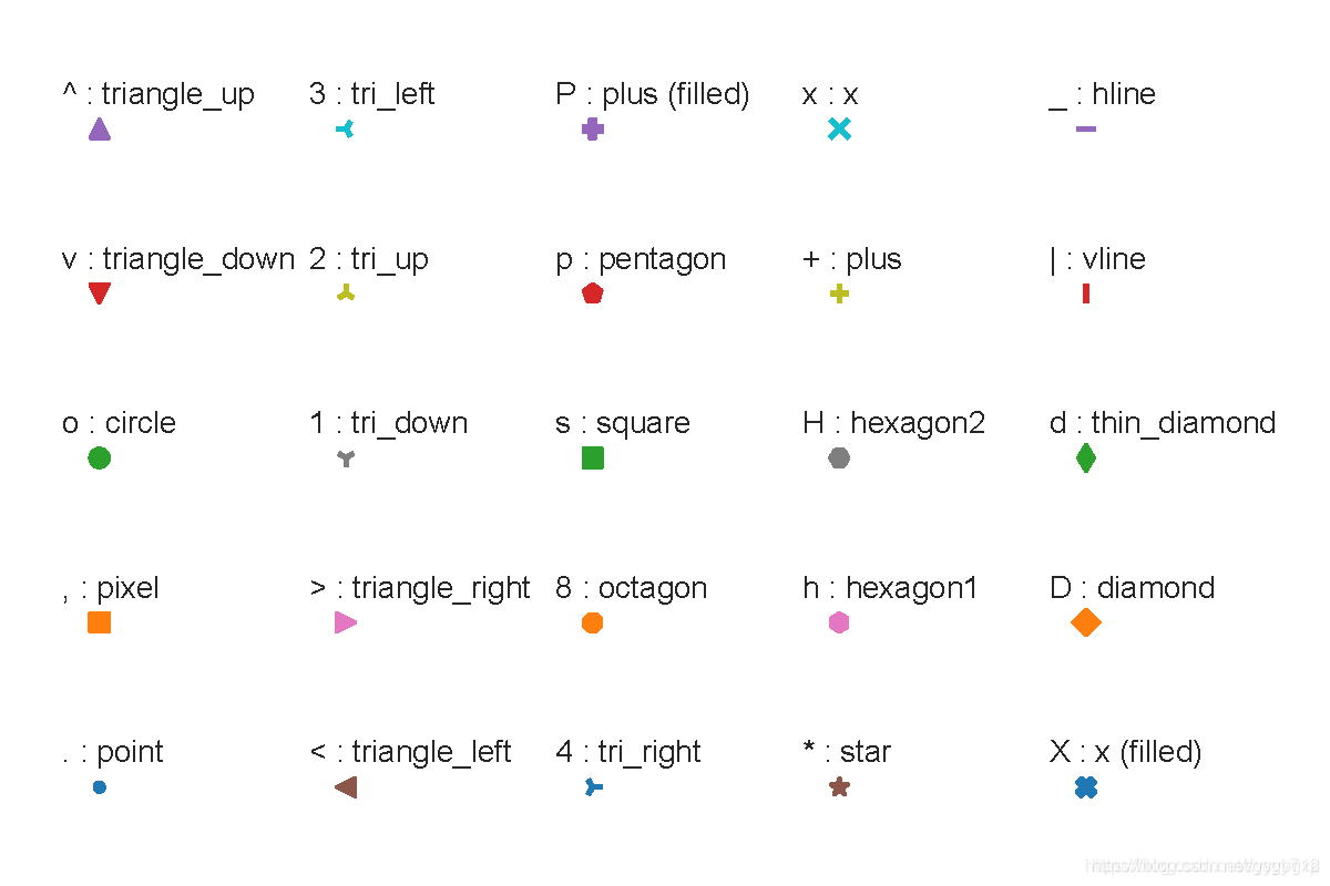
marker可选参数

'.'       point marker
','       pixel marker
'o'       circle marker
'v'       triangle_down marker
'^'       triangle_up marker
'<'       triangle_left marker
'>'       triangle_right marker
'1'       tri_down marker
'2'       tri_up marker
'3'       tri_left marker
'4'       tri_right marker
's'       square marker
'p'       pentagon marker
'*'       star marker
'h'       hexagon1 marker
'H'       hexagon2 marker
'+'       plus marker
'x'       x marker
'D'       diamond marker
'd'       thin_diamond marker
'|'       vline marker
'_'       hline marker

在这里插入图片描述

可选颜色
Python作图颜色汇总

常用设置，参考文章

import matplotlib.pyplot as plt
from matplotlib.pyplot import figure
import numpy as np

figure(num=None, figsize=(2.8, 1.7), dpi=300)
# figsize的2.8和1.7指的是英寸，dpi指定图片分辨率。那么图片就是（2.8*300）*（1.7*300）像素大小

plt.plot(test_mean_1000S_n, 'royalblue', label='without threshold')
plt.plot(test_mean_1000S, 'darkorange', label='with threshold')
# 画图，并指定颜色

plt.xticks(fontproperties = 'Times New Roman', fontsize=8)
plt.yticks(np.arange(0, 1.1, 0.2), fontproperties = 'Times New Roman', fontsize=8)
# 指定横纵坐标的字体以及字体大小，记住是fontsize不是size。yticks上我还用numpy指定了坐标轴的变化范围。

plt.legend(loc='lower right', prop={'family':'Times New Roman', 'size':8})
# 图上的legend，记住字体是要用prop以字典形式设置的，而且字的大小是size不是fontsize，这个容易和xticks的命令弄混

plt.title('1000 samples', fontdict={'family' : 'Times New Roman', 'size':8})
# 指定图上标题的字体及大小

plt.xlabel('iterations', fontdict={'family' : 'Times New Roman', 'size':8})
plt.ylabel('accuracy', fontdict={'family' : 'Times New Roman', 'size':8})
# 指定横纵坐标描述的字体及大小

plt.savefig('F:/where-you-want-to-save.png', dpi=300, bbox_inches="tight")
# 保存文件，dpi指定保存文件的分辨率
# bbox_inches="tight" 可以保存图上所有的信息，不会出现横纵坐标轴的描述存掉了的情况

plt.show()
# 记住，如果你要show()的话，一定要先savefig，再show。如果你先show了，存出来的就是一张白纸。

网格设置

链接：https://www.jianshu.com/p/e59bcd5324f1
matplotlib.pyplot.grid(b, which, axis, color, linestyle, linewidth， **kwargs)

b : 布尔值。就是是否显示网格线的意思。官网说如果b设置为None，且kwargs长度为0，则切换网格状态。

which : 取值为’major’, ‘minor’， ‘both’。默认为’major’。

axis : 取值为‘both’， ‘x’，‘y’。就是想绘制哪个方向的网格线。

color : 这就不用多说了，就是设置网格线的颜色。或者直接用c来代替color也可以。

linestyle :也可以用ls来代替linestyle，设置网格线的风格，是连续实线，虚线或者其它不同的线条。 | ‘-’ |
‘–’ | ‘-.’ | ‘:’ | ‘None’ | ‘’ | ‘’]

linewidth : 设置网格线的宽度

边框与坐标轴设置

参考文章

ax.spines['top'].set_visible(False)   # 隐藏部分边框
ax.spines['right'].set_visible(False)

ax.set_yticks([1,2,3,4])  # 自定义刻度

坐标轴范围设置——只设置一侧

ylim(top=3)  # adjust the top leaving bottom unchanged
ylim(bottom=1)  # adjust the bottom leaving top unchanged
xlim(right=3)  # adjust the right leaving left unchanged
xlim(left=1)  # adjust the left leaving right unchanged

设置横纵坐标比例相同

ax1.set_aspect('equal', adjustable='box')

设置刻度方向向内/外

ax.tick_params(axis="y", direction="in", which="minor", length=4)
ax.tick_params(axis="y", direction="out", which="major", labelsize=15, length=5)

参考文章
https://blog.csdn.net/gsgbgxp/article/details/125077492
https://blog.csdn.net/Admiral_x/article/details/124778091
https://blog.csdn.net/wyy74389/article/details/120828086

图例设置

关于图例参数的较为完整的介绍 https://www.jb51.net/article/191933.htm
1、保存画布外图例
如何将画布外的图例也保存进来？参考文章 https://www.jb51.net/article/191919.htm
里面介绍了多种方法，最后自己采用的是在 savefig 时加上一句 bbox_inches='tight

fig.savefig('scatter2.png',dpi=600,bbox_inches='tight')

2、图例位置设置
这方面网上博客很多，随手就能搜到。

'best'         : 0, (only implemented for axes legends)
'upper right'  : 1,
'upper left'   : 2,
'lower left'   : 3,
'lower right'  : 4,
'right'        : 5,
'center left'  : 6,
'center right' : 7,
'lower center' : 8,
'upper center' : 9,
'center'       : 10,

如果想自定义位置也很简单，loc=(0.2,0.8)即代表在画布的横纵比例位置。
此外，loc 参数还经常和bbox_to_anchor参数组合，具体用法参考链接
https://blog.csdn.net/Wannna/article/details/102751689
https://blog.csdn.net/Gou_Hailong/article/details/121795267
https://matplotlib.org/stable/api/legend_api.html
下面给出示例

l1 = plt.legend(bbox_to_anchor=(1.04,1), borderaxespad=0)
l2 = plt.legend(bbox_to_anchor=(1.04,0), loc="lower left", borderaxespad=0)
l3 = plt.legend(bbox_to_anchor=(1.04,0.5), loc="center left", borderaxespad=0)
l4 = plt.legend(bbox_to_anchor=(0,1.02,1,0.2), loc="lower left",
                mode="expand", borderaxespad=0, ncol=3)
l5 = plt.legend(bbox_to_anchor=(1,0), loc="lower right", 
                bbox_transform=fig.transFigure, ncol=3)
l6 = plt.legend(bbox_to_anchor=(0.4,0.8), loc="upper right")

作图结果
在这里插入图片描述
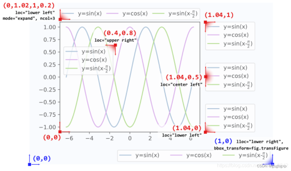
如果 bbox_to_anchor 单独使用，那就是以图左下角为基准。
如果和 loc 配合使用，则 loc 指明的是图例的哪个角，比如 bbox_to_anchor=(0.4,0.8), loc="upper right" 的意思就是把图例的右上角放置在图的 (0.4,0.8) 的位置上。
如果 bbox_to_anchor 用的是四元素，则

it specifies the bbox (x, y, width, height) that the legend is placed in. To put the legend in the best location in the bottom right quadrant of the axes (or figure):

loc='best', bbox_to_anchor=(0.5, 0., 0.5, 0.5)

其实是创建了一个新的图框bbox，图框的位置由前两个元素决定，大小由后两个元素决定，都是相对原图而言，如后两个元素都是0.5就意味着长宽都是原图的一半。然后loc定义的是在这个图框bbox中的位置。

添加箭头与文本框

1、添加箭头
箭头的标注用到 annotate，但设置参数较多，这里只给出几个比较靠谱的链接，之后用到随时查吧。
添加箭头参考文章

《Python数据科学手册》4.11.3节
https://blog.csdn.net/qq_21478261/article/details/108290310
https://www.cnblogs.com/-wenli/p/12854766.html
https://www.cnblogs.com/dqi1999/articles/14004235.html
https://blog.csdn.net/qq_30638831/article/details/79938967
官方文档 FancyArrowPatch、ArrowStyle

需要注意的是如果设置了 arrowstyle，那箭头的宽度长度是在定义 arrowstyle 时一并定义的，而不是在 arrowprops 里定义的。例如

ax1.annotate('', xy=(60,50), xytext=(110,50), arrowprops=dict(facecolor='brown', 
			 shrink=0.05, alpha=0.5, width=10, headtength=20, headwidth=25))
ax1.annotate('', xy=(60,50), xytext=(110,50), 
			 arrowprops=dict(arrowstyle="fancy, head length=3, head width=3, tail width=2", 
			 ec="none", color=' chocolate', alpha=0.7)

2、添加文本

参考文章

ax2.text(80,47,'The\ntext', size=10, ha='center', linespacing = 1.5,
		 bbox=dict(boxstyle="round", ec="none", color='chocolate', alpha=0.7))

图片保存、关闭

参考链接

   clf() # 清图。
   cla() # 清坐标轴。
   close() # 关窗口

fig = plt.figure(0) # 新图 0
plt.savefig() # 保存
plt. close(0) # 关闭图 0

fig = plt.figure() # 新图 0
plt.savefig() # 保存
plt.close('all') # 关闭图 0

图片保存用到的函数是savefig，官方链接：matplotlib.pyplot.savefig
调用格式为

savefig(fname, *, dpi='figure', format=None, metadata=None,
        bbox_inches=None, pad_inches=0.1,
        facecolor='auto', edgecolor='auto',
        backend=None, **kwargs
       )

其中pad_inches表示保存图片时周边的留白，默认值为0.1，不过设为0可能更适合于论文。
图片保存需要设置分辨率和保存格式的时候写为

fig = plt.figure(figsize=(12,4))
fig.savefig('AAA.eps',dpi=600)   # dpi一般300足够，再高可设为600、1200

如果涉及到用Python作图保存的图矢量格式为svg、eps、pdf的，不能直接插入word的问题（Word本身只能接受wmf，emf格式的矢量图），可以参考文章。
后来发现2019版的Word是可以插入svg的，这样就不需要转换图片格式了。
但是在LaTeX中编译似乎svg不是一个很好的格式（见文章Latex 插入矢量图）。在LaTeX中似乎更推荐 pdf 和 eps。
有时如果需要把图片转换为svg格式的话，可以在Convertio网站上完成。

其他

风格设置

matplotlib也可以像Seaborn那样设置绘图风格

import matplotlib.pyplot as plt
plt.style.use('ggplot')

画布颜色

参考链接：https://zhuanlan.zhihu.com/p/215883403
画布的背景颜色设置

fig = plt.figure(figsize=(15,12),facecolor='black',edgecolor='black')
ax = fig.add_subplot()

figsize参数表示画布大小，facecolor表示画布颜色设置，edgecolor表示画布边线颜色设置，运行上述代码，可以得到
绘图区的颜色设置

ax.patch.set_facecolor("green") # 设置 ax1 区域背景颜色
ax.patch.set_alpha(0.5) # 设置 ax1 区域背景颜色透明度

对数坐标轴

在网上看了很多方案，还是直接设置最方便，搭配plt.style.use('ggplot')使用，显示效果更佳。

ax1.set_xscale('log')

其他方法可以参考链接：https://www.jianshu.com/p/8c370f0dcef8
这其中使用semilogx和semilogy应该也是不错的选择。
semilogy的官方说明：https://matplotlib.org/3.3.0/api/_as_gen/matplotlib.pyplot.semilogy.html

局部放大图

参考链接 https://blog.csdn.net/wulishinian/article/details/106668011

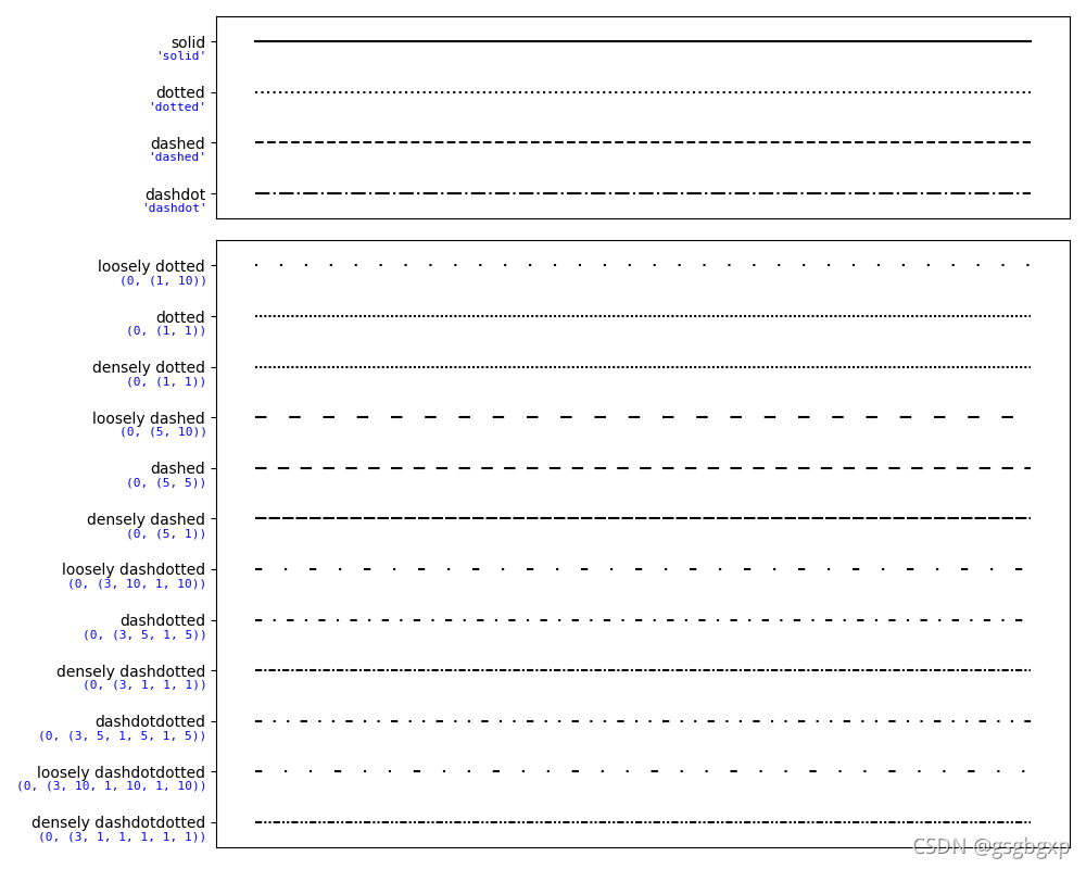
所有线型

参考链接 https://matplotlib.org/3.1.1/gallery/lines_bars_and_markers/linestyles.html?highlight=linestyle
注意下面这些特殊线型在使用时是输入数组，例如 linestyle=(0, (1, 10)) 而不是 linestyle='loosely dotted'

import numpy as np
import matplotlib.pyplot as plt

linestyle_str = [
     ('solid', 'solid'),      # Same as (0, ()) or '-'
     ('dotted', 'dotted'),    # Same as (0, (1, 1)) or '.'
     ('dashed', 'dashed'),    # Same as '--'
     ('dashdot', 'dashdot')]  # Same as '-.'

linestyle_tuple = [
     ('loosely dotted',        (0, (1, 10))),
     ('dotted',                (0, (1, 1))),
     ('densely dotted',        (0, (1, 1))),

     ('loosely dashed',        (0, (5, 10))),
     ('dashed',                (0, (5, 5))),
     ('densely dashed',        (0, (5, 1))),

     ('loosely dashdotted',    (0, (3, 10, 1, 10))),
     ('dashdotted',            (0, (3, 5, 1, 5))),
     ('densely dashdotted',    (0, (3, 1, 1, 1))),

     ('dashdotdotted',         (0, (3, 5, 1, 5, 1, 5))),
     ('loosely dashdotdotted', (0, (3, 10, 1, 10, 1, 10))),
     ('densely dashdotdotted', (0, (3, 1, 1, 1, 1, 1)))]


def plot_linestyles(ax, linestyles):
    X, Y = np.linspace(0, 100, 10), np.zeros(10)
    yticklabels = []

    for i, (name, linestyle) in enumerate(linestyles):
        ax.plot(X, Y+i, linestyle=linestyle, linewidth=1.5, color='black')
        yticklabels.append(name)

    ax.set(xticks=[], ylim=(-0.5, len(linestyles)-0.5),
           yticks=np.arange(len(linestyles)), yticklabels=yticklabels)

    # For each line style, add a text annotation with a small offset from
    # the reference point (0 in Axes coords, y tick value in Data coords).
    for i, (name, linestyle) in enumerate(linestyles):
        ax.annotate(repr(linestyle),
                    xy=(0.0, i), xycoords=ax.get_yaxis_transform(),
                    xytext=(-6, -12), textcoords='offset points',
                    color="blue", fontsize=8, ha="right", family="monospace")


fig, (ax0, ax1) = plt.subplots(2, 1, gridspec_kw={'height_ratios': [1, 3]},
                               figsize=(10, 8))

plot_linestyles(ax0, linestyle_str[::-1])
plot_linestyles(ax1, linestyle_tuple[::-1])

plt.tight_layout()
plt.show()