关联规则之Apriori算法

Apriori算法（调包实现）

算法简单描述：

两个重要参数：
1、频繁项集(frequent item sets)。包括计算：频繁项集的支持度（support）
2、关联规则(association rules)。包括计算：关联规则的置信度(confidence)

频繁项集(frequent item sets)，支持度（support）

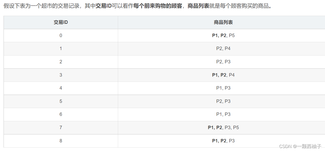
单是肉眼去观察的话，似乎顾客经常购买P1, P2这样的组合。这种的购物中出现的经常的组合，就是我们要找的频繁项集了。项集可以由一个商品组成，也可以由多个商品组成。比如{P1}是一个项集，{P1, P2}也是一个项集。因此这里的有个最小支持度阈值，改项集的概率大于最小支持度时，即可以称该项集为频繁项集。

频繁项集的特点：

频繁项集拥有如下特点：**如果某个项集是频繁的，那么它的所有子集也是频繁的。**比如项集{P1, P2}是频繁的，那么项集{P1}和{P2}也是频繁的。该原理倒过来推并不成立，也就是说当我们 只发现{P1}和{P2}是频繁的的时候，是无法推出项集{P1, P2}是频繁的，因为有可能他们的频繁是依靠和别的商品一起购买组合而成的。这样已知项集{2，3}是非频繁的。利用这个知识，我们就知道项集{0,2,3} ，{1,2,3}以及{0,1,2,3}也是非频繁的。该特点的最大用处是帮助我们减少计算。

关联规则(association rules)置信度(confidence)

我们的目的是根据频繁项集挖掘出关联规则。关联规则的意思就是通过某个项集可以推导出另一个项集。比如一个频繁项集{P1, P2, P3}，就可以推导出六个可能的关联规则。其中置信度最高的就是最有可能的关联规则。
{P1} → {P2, P3}
{P2} → {P1, P3}
{P2} → {P1, P3}
{P3} → {P1, P2}
{P1, P2} → {P3}
{P2, P3} → {P1}
{P1, P3} → {P2}
强关联规则满足：
confidence(A ⇒ B)>min_Support
confidence(A ⇒ B) = Support(A⇒B) /Support(A) ≥ min_confidence

具体问题

问题描述，某天早上在你的班上收集10个学生的早餐，最小支持阈值= 0.2，最小置信阈值= 0.8。早餐项目来源包括:包子、油条、馒头、鸡蛋、面包、咖啡、果汁、牛奶、豆浆等。
准备数据：

item_list = [[‘milk’, ‘bread’],
[‘milk’, ‘bread’,‘juice’],
[‘juice’, ‘bread’,‘egg’],
[‘milk’, ‘bread’],
[‘soybean_mil’,‘bread’],
[‘soybean_mil’, ‘baozi’],
[‘milk’, ‘bread’, ‘egg’],
[‘milk’, ‘bread’,‘egg’],
[‘mantou’,‘juice’, ‘milk’],
[‘bread’, ‘milk’, ‘egg’]]
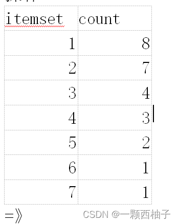
对不同早餐进行统计和编号，便于后面进行书写和统计
bread 8;milk 7 ;egg 4;juice 3;soybean_milk 2;baozi 1;mantou 1;
进行编号，依次为 1，2，3，4，5，6，7
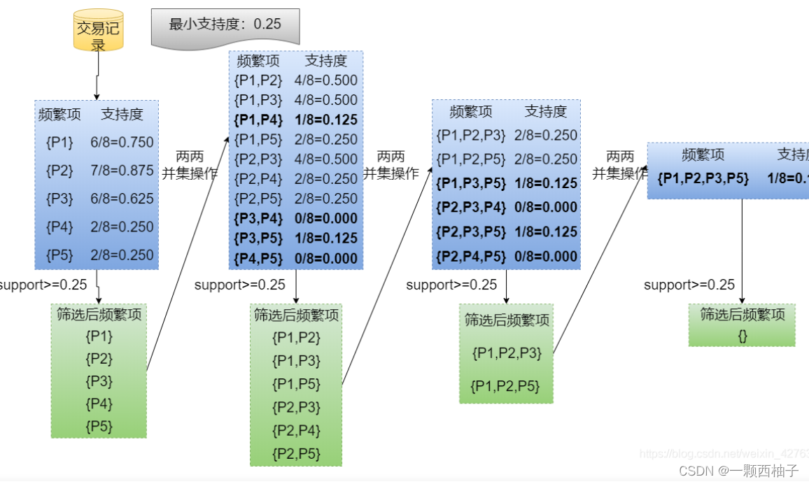
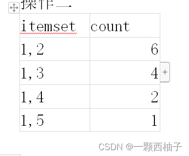
找出frequent itemset
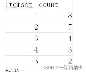
因为minimum support threshold = 0.2，

去掉小于最小支持度的

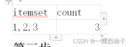
依次做下去：
最后结果

根据：confidence(A ⇒ B) = Support(A⇒B) Support(A) ≥ min_conf
min_conf=0.8
Support({i1,i2,i3}) /Support({i1}) = 3 / 8= 37.5% < 80%
Support({i1,i2,i3}) /Support({i2}) = 3 / 7= 42.8% < 80%
Support({i1,i2,i3}) /Support({i3}) = 3 / 4= 75% < 80%
Support({i1,i2,i3}) /Support({i1,i2}) = 3 / 6= 50% < 80%
Support({i1,i2,i3}) /Support({i1,3}) = 3 / 4= 75% < 80%
Support({i1,i2,i3}) /Support({i2,i3}) = 3 / 3= 100% > 80%
Support({i1,i2,i3}) /Support({i1,i2,i3}) = 3 / 3= 100% > 80%
得出强关联规则
output a strong association rules {i2, i3} ⇒ i1

import pandas as pd
import numpy as np

# 设置显示的最大列、宽等参数，消掉打印不完全中间的省略号
pd.set_option('display.max_columns', 1000)
pd.set_option('display.width', 1000)
pd.set_option('display.max_colwidth', 1000)
# 设置数据集
item_list = [['milk', 'bread'],
   ['milk', 'bread','juice'],
   ['juice', 'bread','egg'],
   ['milk', 'bread'],
   ['soybean_mil','bread'],
   ['soybean_mil', 'baozi'],
   ['milk', 'bread', 'egg'],
   ['milk', 'bread','egg'],
   ['mantou','juice', 'milk'],
   ['bread', 'milk', 'egg']]
# 进行编号后的早餐数据
'''
    对不同早餐进行统计和编号，便于后面进行书写和统计
    bread 8;milk 7 ;egg 4;juice 3;soybean_milk 2;baozi 1;mantou 1;
    进行编号，依次为 1，2，3，4，5，6，7
    '''
# item_list = [['2', '1'],
#             ['2', '1','4'],
#             ['4', '1','3'],
#             ['2', '1'],
#             ['5','1'],
#             ['5', '6'],
#             ['2', '1', '3'],
#             ['2', '1','3'],
#             ['7','4', '2'],
#             ['1', '2', '3']]

item_df = pd.DataFrame(item_list)

from mlxtend.preprocessing import TransactionEncoder

te = TransactionEncoder()
df_tf = te.fit_transform(item_list)
df = pd.DataFrame(df_tf, columns=te.columns_)
# 计算频繁项集
from mlxtend.frequent_patterns import apriori

# use_colnames=True表示使用元素名字，默认的False使用列名代表元素, 设置最小支持度min_support
frequent_itemsets = apriori(df, min_support=0.2, use_colnames=True)

frequent_itemsets.sort_values(by='support', ascending=False, inplace=True)

# 选择2频繁项集,len(x)==3,表示三种不同早餐组成的集合
print(frequent_itemsets[frequent_itemsets.itemsets.apply(lambda x: len(x)) == 3])
print(frequent_itemsets[frequent_itemsets.itemsets.apply(lambda x: len(x)) == 2])

# 计算关联规则
from mlxtend.frequent_patterns import association_rules

# metric可以有很多的度量选项，返回的表列名都可以作为参数
association_rule = association_rules(frequent_itemsets, metric='confidence', min_threshold=0.8)

# 关联规则可以提升度排序
association_rule.sort_values(by=['confidence','lift'], ascending=False, inplace=True)
print(association_rule)

# 规则是：antecedents->consequents