高光谱图像噪声检测及光谱曲线平滑（1）Savitzky Golay Filtering滤波

Savitzky-Golay-Smoothers是线性滤波器，用于平滑数据或计算给定顺序的平滑导数，并保留底层信号的峰值和其他重要特征。

举个例子

#!python
def savitzky_golay(y, window_size, order, deriv=0, rate=1):
    r"""Smooth (and optionally differentiate) data with a Savitzky-Golay filter.
    The Savitzky-Golay filter removes high frequency noise from data.
    It has the advantage of preserving the original shape and
    features of the signal better than other types of filtering
    approaches, such as moving averages techniques.
    Parameters
    ----------
    y : array_like, shape (N,)
        the values of the time history of the signal.
    window_size : int
        the length of the window. Must be an odd integer number.
    order : int
        the order of the polynomial used in the filtering.
        Must be less then `window_size` - 1.
    deriv: int
        the order of the derivative to compute (default = 0 means only smoothing)
    Returns
    -------
    ys : ndarray, shape (N)
        the smoothed signal (or it's n-th derivative).
    Notes
    -----
    The Savitzky-Golay is a type of low-pass filter, particularly
    suited for smoothing noisy data. The main idea behind this
    approach is to make for each point a least-square fit with a
    polynomial of high order over a odd-sized window centered at
    the point.
    Examples
--------
    t = np.linspace(-4, 4, 500)
    y = np.exp( -t**2 ) + np.random.normal(0, 0.05, t.shape)
    ysg = savitzky_golay(y, window_size=31, order=4)
    import matplotlib.pyplot as plt
    plt.plot(t, y, label='Noisy signal')
    plt.plot(t, np.exp(-t**2), 'k', lw=1.5, label='Original signal')
    plt.plot(t, ysg, 'r', label='Filtered signal')
    plt.legend()
    plt.show()
    References
    ----------
    .. [1] A. Savitzky, M. J. E. Golay, Smoothing and Differentiation of
       Data by Simplified Least Squares Procedures. Analytical
       Chemistry, 1964, 36 (8), pp 1627-1639.
    .. [2] Numerical Recipes 3rd Edition: The Art of Scientific Computing
       W.H. Press, S.A. Teukolsky, W.T. Vetterling, B.P. Flannery
       Cambridge University Press ISBN-13: 9780521880688
    """
import numpy as np
    from math import factorial

    try:
        window_size = np.abs(np.int(window_size))
        order = np.abs(np.int(order))
    except ValueError, msg:
        raise ValueError("window_size and order have to be of type int")
    if window_size % 2 != 1 or window_size < 1:
        raise TypeError("window_size size must be a positive odd number")
    if window_size < order + 2:
        raise TypeError("window_size is too small for the polynomials order")
    order_range = range(order+1)
    half_window = (window_size -1) // 2
    # precompute coefficients
    b = np.mat([[k**i for i in order_range] for k in range(-half_window, half_window+1)])
    m = np.linalg.pinv(b).A[deriv] * rate**deriv * factorial(deriv)
    # pad the signal at the extremes with
    # values taken from the signal itself
    firstvals = y[0] - np.abs( y[1:half_window+1][::-1] - y[0] )
    lastvals = y[-1] + np.abs(y[-half_window-1:-1][::-1] - y[-1])
    y = np.concatenate((firstvals, y, lastvals))
    return np.convolve( m[::-1], y, mode='valid')

代码解释在第61-62行中，预先计算局部最小二乘多项式拟合的系数。 这些将在稍后的第68行使用，它们将与信号相关。 为了防止数据极端的假结果，信号的两端用镜像填充（第65-67行）。

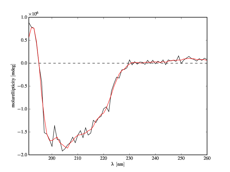
蛋白质的CD谱。 黑色：原始数据。 红色：应用过滤器后的曲线

循环伏安数据的封装 S-G滤光片最受欢迎的应用之一，除了平滑的UV-VIS和IR光谱之外，还使得电分析实验中获得的曲线平滑。 在循环伏安法中，电压（作为abcissa）像三角波一样变化。 而在信号中，在转折点（切换电位）处有尖角，这是不应平滑的。 在这种情况下，Savitzky-Golay平滑应该分段进行，即。 单独的片断在x单调：

#!python numbers=disable
def savitzky_golay_piecewise(xvals, data, kernel=11, order =4):
    turnpoint=0
    last=len(xvals)
    if xvals[1]>xvals[0] : #x is increasing?
        for i in range(1,last) : #yes
            if xvals[i]<xvals[i-1] : #search where x starts to fall
                turnpoint=i
                break
    else: #no, x is decreasing
        for i in range(1,last) : #search where it starts to rise
            if xvals[i]>xvals[i-1] :
                turnpoint=i
                break
    if turnpoint==0 : #no change in direction of x
        return savitzky_golay(data, kernel, order)
    else:
        #smooth the first piece
        firstpart=savitzky_golay(data[0:turnpoint],kernel,order)
        #recursively smooth the rest
        rest=savitzky_golay_piecewise(xvals[turnpoint:], data[turnpoint:], kernel, order)
        return numpy.concatenate((firstpart,rest))

二维数据平滑和最小二乘梯度估计
Savitsky-Golay滤波器也可用于平滑受噪声影响的二维数据。该算法与一维情况完全相同，只有数学有点棘手。基本算法如下：1.对于二维矩阵的每一个点，提取一个以该点为中心，大小等于奇数“window_size”的子矩阵。 2.对于这个子矩阵，计算多项式曲面的最小二乘拟合，定义为p（x，y）= a0 + a1 * x + a2 * y + a3 * x \ ^ 2 + a4 * y \ ^ 2 + a5 * x * y + ...。请注意，x和y在中心点等于零。 3.用适合值计算的值替换初始中心点。
请注意，由于拟合系数相对于数据间距是线性的，因此可以预先计算效率。此外，重要的是适当填充数据的边界与数据本身的镜像，以便对数据边界处拟合的评估能够顺利进行。
这里是二维过滤的代码。

#!python numbers=enable
def sgolay2d ( z, window_size, order, derivative=None):
    """
    """
    # number of terms in the polynomial expression
    n_terms = ( order + 1 ) * ( order + 2)  / 2.0

    if  window_size % 2 == 0:
        raise ValueError('window_size must be odd')

    if window_size**2 < n_terms:
        raise ValueError('order is too high for the window size')

    half_size = window_size // 2

    # exponents of the polynomial. 
    # p(x,y) = a0 + a1*x + a2*y + a3*x^2 + a4*y^2 + a5*x*y + ... 
    # this line gives a list of two item tuple. Each tuple contains 
    # the exponents of the k-th term. First element of tuple is for x
    # second element for y.
    # Ex. exps = [(0,0), (1,0), (0,1), (2,0), (1,1), (0,2), ...]
    exps = [ (k-n, n) for k in range(order+1) for n in range(k+1) ]

    # coordinates of points
    ind = np.arange(-half_size, half_size+1, dtype=np.float64)
    dx = np.repeat( ind, window_size )
    dy = np.tile( ind, [window_size, 1]).reshape(window_size**2, )

    # build matrix of system of equation
    A = np.empty( (window_size**2, len(exps)) )
    for i, exp in enumerate( exps ):
        A[:,i] = (dx**exp[0]) * (dy**exp[1])
 # pad input array with appropriate values at the four borders
    new_shape = z.shape[0] + 2*half_size, z.shape[1] + 2*half_size
    Z = np.zeros( (new_shape) )
    # top band
    band = z[0, :]
    Z[:half_size, half_size:-half_size] =  band -  np.abs( np.flipud( z[1:half_size+1, :] ) - band )
    # bottom band
    band = z[-1, :]
    Z[-half_size:, half_size:-half_size] = band  + np.abs( np.flipud( z[-half_size-1:-1, :] )  -band )
    # left band
    band = np.tile( z[:,0].reshape(-1,1), [1,half_size])
    Z[half_size:-half_size, :half_size] = band - np.abs( np.fliplr( z[:, 1:half_size+1] ) - band )
    # right band
    band = np.tile( z[:,-1].reshape(-1,1), [1,half_size] )
    Z[half_size:-half_size, -half_size:] =  band + np.abs( np.fliplr( z[:, -half_size-1:-1] ) - band )
    # central band
    Z[half_size:-half_size, half_size:-half_size] = z

    # top left corner
    band = z[0,0]
    Z[:half_size,:half_size] = band - np.abs( np.flipud(np.fliplr(z[1:half_size+1,1:half_size+1]) ) - band )
    # bottom right corner
    band = z[-1,-1]
    Z[-half_size:,-half_size:] = band + np.abs( np.flipud(np.fliplr(z[-half_size-1:-1,-half_size-1:-1]) ) - band )

    # top right corner
    band = Z[half_size,-half_size:]
    Z[:half_size,-half_size:] = band - np.abs( np.flipud(Z[half_size+1:2*half_size+1,-half_size:]) - band )
    # bottom left corner
    band = Z[-half_size:,half_size].reshape(-1,1)
    Z[-half_size:,:half_size] = band - np.abs( np.fliplr(Z[-half_size:, half_size+1:2*half_size+1]) - band )
# solve system and convolve
    if derivative == None:
        m = np.linalg.pinv(A)[0].reshape((window_size, -1))
        return scipy.signal.fftconvolve(Z, m, mode='valid')
    elif derivative == 'col':
        c = np.linalg.pinv(A)[1].reshape((window_size, -1))
        return scipy.signal.fftconvolve(Z, -c, mode='valid')
    elif derivative == 'row':
        r = np.linalg.pinv(A)[2].reshape((window_size, -1))
        return scipy.signal.fftconvolve(Z, -r, mode='valid')
    elif derivative == 'both':
        c = np.linalg.pinv(A)[1].reshape((window_size, -1))
        r = np.linalg.pinv(A)[2].reshape((window_size, -1))
        return scipy.signal.fftconvolve(Z, -r, mode='valid'), scipy.signal.fftconvolve(Z, -c, mode='valid')

这里有个例子

#!python number=enable

# create some sample twoD data
x = np.linspace(-3,3,100)
y = np.linspace(-3,3,100)
X, Y = np.meshgrid(x,y)
Z = np.exp( -(X**2+Y**2))

# add noise
Zn = Z + np.random.normal( 0, 0.2, Z.shape )

# filter it
Zf = sgolay2d( Zn, window_size=29, order=4)

# do some plotting
matshow(Z)
matshow(Zn)
matshow(Zf)

附件：Original.pdf原始数据附件：Original + noise.pdf原始数据+噪声附件：Original + noise + filtered.pdf（原始数据+噪声）过滤

二维函数的渐变
由于我们已经计算了最佳的拟合插值多项式曲面，所以很容易计算其梯度。 这种计算二维函数梯度的方法是相当稳健的，部分地隐藏了数据中的噪声，这强烈地影响了分化操作。 可以明显计算的导数的最大阶数取决于拟合中使用的多项式的阶数。
上面提供的代码有一个选项导数，它现在允许计算二维数据的一阶导数。 它可以是“行”或“列”，表示导数的方向，或“两者”，它返回的梯度。

本文来自

http://scipy-cookbook.readthedocs.io/items/SavitzkyGolay.html

For further information see: http://www.wire.tu-bs.de/OLDWEB/mameyer/cmr/savgol.pdf

(or http://www.dalkescientific.com/writings/NBN/data/savitzky_golay.py for a pre-numpy implementation).