Random Forests C++实现：细节，使用与实验

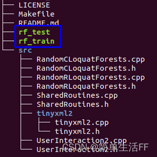
项目主页：randomforest github, gitee
C++ implementation of random forests classification, regression, proximity and variable importance.
欢迎讨论

          _____                 _                 ______                  _
         |  __ \               | |               |  ____|                | |
         | |__) |__ _ _ __   __| | ___  _ __ ___ | |__ ___  _ __ ___  ___| |_
         |  _  // _` | '_ \ / _` |/ _ \| '_ ` _ \|  __/ _ \| '__/ _ \/ __| __|
         | | \ \ (_| | | | | (_| | (_) | | | | | | | | (_) | | |  __/\__ \ |_
         |_|  \_\__,_|_| |_|\__,_|\___/|_| |_| |_|_|  \___/|_|  \___||___/\__|

1. 随机森林简介

1.1 算法简介

        随机森林（Random Forest, RF）算法是一类集成学习算法，它由统计学习界的大师级人物 Leo Breiman(1928–2005) 提出^[1]。它是若干随机树（Randomized Tree）的组合，这些随机树彼此互相独立，而且在训练样本的选择和树的生长过程中引入随机性以降低树结构分类器较高的方差。随机森林在很多应用场景下具有不错的准确性，它具备一些优良特性，比如，较少的超参，高效的训练与预测，多分类和对噪声不敏感等。这些特性使它广泛应用于不同领域，比如计算机视觉，遥感，生物信息学等。特别在计算机视觉领域，随机森林在图像分割、特征点识别、目标检测和人体部件识别等方面都有比较成功的应用。
        本文并不是随机森林算法的入门，需要对RF算法具有一定的认识甚至实践经验。若想对RF有详细甚至进一步的深入了解，推荐阅读微软的技术报告^[3]，这份报告对分类森林、随机回归森林、概率密度森林等从算法和实现角度进行了介绍。也可以参考Gilles Louppe的博士论文，作者对实现细节做了非常详尽的描述^[7]。

1.2 随机特性

        针对不同问题随机森林学习算法包括分类和回归两类。随机森林是一组随机树的组合，它们彼此独立且有较大差异。其中的随机树按传统分类回归树(Classification and Regression Tree, CART) 的训练方式生长到最大深度，但是不进行剪枝（pruning）。随机性主要体现在两个方面：（1）训练样本的随机选择，即使用自举重采样法（Bootstrap Sampling）为森林中每棵树生成有差异的训练样本，其本质上是 Bagging 集成学习思想。Bagging 能够提高不稳定学习算法分类和预测的准确性，即降低学习算法的方差（Variance）。因此，引入 Bagging方法可降低树结构学习算法较高的方差^[4]。（2）另一方面，随机性也体现在树中节点的分裂方式中。每个节点进行分裂时仅从参数空间中随机选择一个子集，在其中选出“最优”的分裂参数。在树的生长过程中加入随机性可以降低它们彼此之间的相关度，从而降低集成学习算法的泛化误差的上限^[1]。

2. C++实现和使用

2.1 动机

        目前Random Forest的实现大多是python、R语言，C++实现存在但比较少，我所知的且好用的仅有opencv, ALGLIB。此外，上述实现一般作为一个机器学习库的一部分，或者需要科学上网才能下载，使用成本稍高。下图总结了各类RF实现。

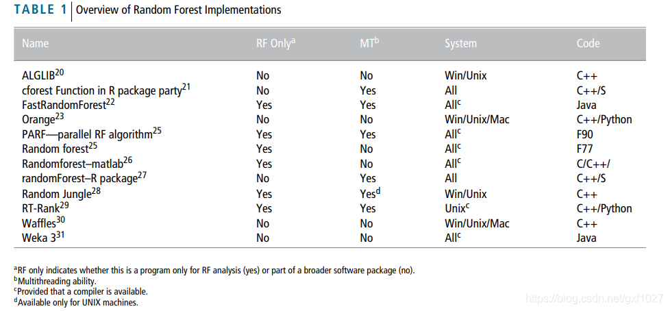
上图来自论文：
Anne-Laure Boulesteix, Silke Janitza. Overview of random forest methodology and practical guidance with emphasis on computational biology and bioinformatics. WIREs Data Mining and Knowledge Discovery 2012, 2: 493–507.
此外，还有微软的decision forest(C++)；刚刚开源的tensorflow决策森林 (TF-DF); 基于NumPy实现的机器学习库 numpy-ml;
高度优化，并且在开源社区中速度最快的scikit-learn中的sklearn.ensemble模块，提供了许多可选参数。
… …

        本文RF实现的主体代码其实在2012年就已经完成，可以用于常规的分类、回归训练，也可以用于实时应用，已经使用过的场景包括目标跟踪（实时训练+分类）、作为实时人脸检测的辅助肤色验证（离线训练+实时分类）。当年还写了篇博文《肤色检测（分割）via Random Forest》，效果还不错。今年3月以来对部分算法和交互的代码做了优化，跑了十几个数据集，并与论文中结果进行了比对，验证了算法的正确性。这版程序尽力做到实现的准确，注重代码质量提高运行性能，兼顾简洁、对用户友好。以下是本RF实现的特点：

1. 适用于分类和回归, 支持回归的多维输出（multi-target regression)
2. 支持3种随机性 (Original RF / Near Original / Extra-Trees)
3. 可计算Proximities，支持离群值计算（raw outlier measure score）
4. 可计算特征重要性
5. 支持OpenMP加速
6. off-the-shelf，即插即用
7. 提供两种使用方式：命令行与嵌入代码(C风格的C++)
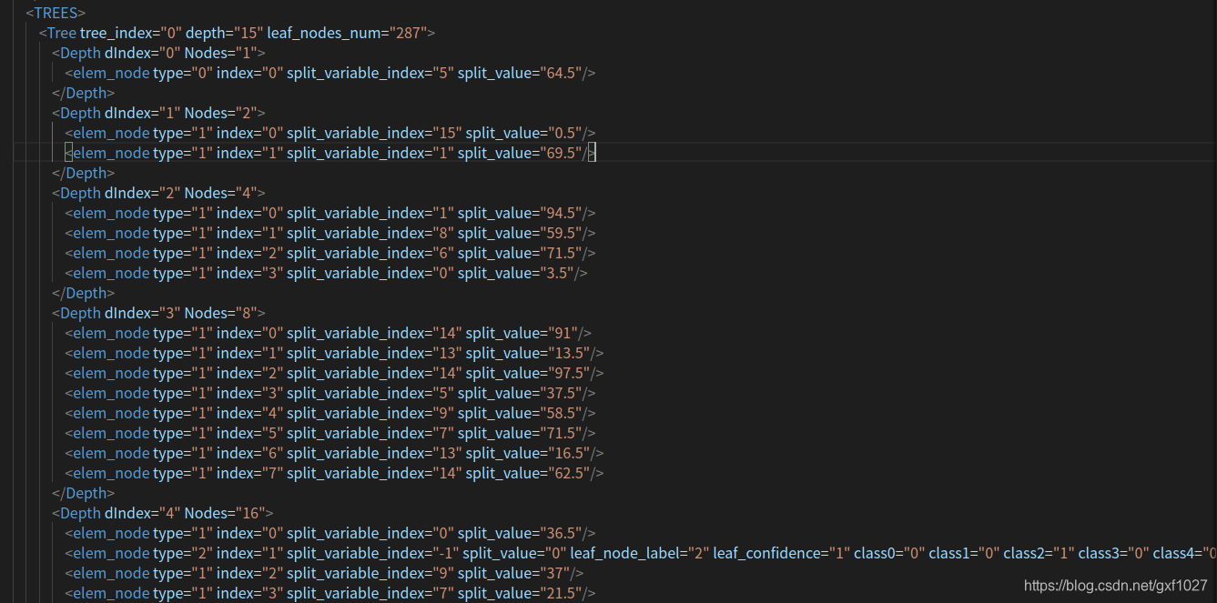
8. 可保存训练完成的模型至本地，也可从本地读取模型。支持两种格式: Plain Text，文件体积小，适用于所有规模的模型；XML格式，可读性强，但不适用于大模型。

2.2 细节

2.2.1 算法的参数（Hyperparameters）

1. MaxDepth: 树最大的深度，若传入负值则使用默认值40
2. TreesNum: 森林中树的数量，若传入负值则使用默认值200
3. SplitVariables: 用于分裂的候选特征数量，如果传入负值则使用默认值，对于分类问题设置为$\sqrt{n\_features}$，对于回归问题设置为$\frac{n\_features}{3}$
4. MinSamplesSplit: 节点还能往下分裂的最小样本数
5. Randomness: 1或2或3，随数字增大在节点分类的随机性增加，1为经典RF（默认），3为Etra-Trees^[4]

2.2.2 关于节点分裂方式

        对于随机森林中的每棵树，在每个节点要寻找“最优”的分裂参数，使训练样本分裂后的信息增益（Information Gain, IG, 式1）最大化。IG衡量了分裂前后节点上样本不纯度（impurity）的下降幅度。对于分类森林，采用了Gini系数来计算节点不纯度；对于回归森林，采用了方差（或协方差）来描述节点不纯度。为了方便实现和控制计算量，采用了“轴平行”（axis aligned）的分裂方式（即经典RF），其他分裂方式可见微软的技术报告^[3]。
$$IG=H\left(S\right)-\sum _{i=l,r}\frac{|S^i|}{|S|}H\left(S^i\right)\text{\hspace{1em}(1)}$$
        上一小节中提到的参数“Randomness”用来控制节点分裂时的随机性，实际上是控制了节点分裂时参数空间的大小，参数空间越小随机性越大。“Randomness”可选参数值为{1，2，3}，对应含义为：

“1”: Breiman的经典RF，在寻找节点分裂特征和分裂值时采用基于优化的快排+“积分”的加速方法，使时间复杂度从$O(n^2)$降低到$O(n\log n)$，$n$为达到节点样本数（实测在elevators数据集上加速370倍，参数为[200, 40, 6, 5]）；
“2”: 从候选特征的最大值与最小值之间均匀得到$K$（默认为50）个候选的分裂值，再从中选择较优的特征和对应的分裂值，当$K\to \infty$，即为经典RF，这个方法grt (github nickgillian / grt)上也被使用；
“3”: 采用论文“Extremely randomized trees”^[4]的方法，从候选特征的最大值与最小值之间随机选择一个值作为候选，然后再选择较优的特征和对应的分裂值。

2.2.3 关于终止条件

当到达节点的样本不可分或者不必再分时，停止树的生长。具体来说，满足以下条件之一时，停止生长，RF不对树进行剪枝。

1. 达到最大深度MaxDepth；
2. 到达节点的样本的不纯度低于阈值：节点上样本的类别相同（适用于分类）或者样本目标值的方差为0（适用于分类回归）；
3. 到达节点的样本数小于等于MinSamplesSplit。
   以上三个条件满足其一，即终止继续生长。
   注：对于分类问题，如果只满足第三个条件，但是最多和第二多类别的样本数相同，那么还需要继续往下生长。

存在特殊情况，当不满足上述“终止条件”，但从候选的SplitVariables个特征中无法获得分裂值，此时尝试从所有特征中随机选择可能的分裂值的方式。这有可能出现在达到节点样本数较少，且SplitVariables较小的场景，恰巧候选特征的值都相同。若还是不可分则停止树的生长。

2.2.4 关于预测

Final predictions are obtained by aggregating over the ensemble. — Gérard Biau

1. 对于分类问题，可用hard descion或者soft decsion两种方式。先介绍后者，随机森林训练结束后，测试样本$x$经过每棵树到达叶子节点，那么样本$x$属于类别$c$的概率为：
   $$p\left(c\mid x\right)=\frac{1}{T}\sum _{t=1}^T{p}_t\left(c\mid x\right)$$
   其中，$T$为森林中随机树的数量，$p_t\left(c\mid x\right)$为叶子节点的类别分布。那么对$x$类别的决策为：
   c ^ = arg ⁡ max ⁡ c ∈ { 1 , ⋯   , N c } p ( c ∣ x ) \hat{c}=\mathop{\arg\max}_{c\in \left \{ 1,\cdots,N_{c} \right \}}p\left ( c\mid x \right ) c^=argmaxc∈{1,⋯,Nc​}​p(c∣x)
   以上是soft decision。对于Hard decision，每颗树输出对应的类别，然后统计出现最多的类别即为$x$的类别，也就是多数投票。

2. 对于回归问题，使用所有树输出的平均值。

2.3 使用

源码可以从github或者gitee项目主页下载

2.3.1 命令行方式

linux:
自行编译

git clone https://github.com/gxf1027/randomforests.git 
(git clone https://gitee.com/gxf1027/randomforests.git)
cd randomforests
# train，生成可执行文件rf_train
make
# test，生成可执行文件rf_test
make -e runtype=test

编译后产生以下两个可执行文件

windows:
包含 src和demo目录下对应文件，通过IDE编译即可。
训练：包含 src目录下所有文件+demo/rf_train.cpp
预测：包含 src目录下所有文件+demo/rf_test.cpp
示例1：训练

分类：./rf_train -p 0 -c RF_config.xml -d dataset.data -o ClassificationForest.xml
回归：./rf_train -p 1 -c RF_config.xml -d dataset.data -o RegressionForest.xml

• -p: '0’表示分类问题，'1’表示回归问题
• -c: RF的参数，通过xml文件指定
  以下为参数文件的示例

<?xml version="1.0" ?>
<RandomForestConfig>
	<MaxDepth>40</MaxDepth>
	<TreesNum>200</TreesNum>
	<SplitVariables>4</SplitVariables>
	<MinSamplesSplit>5</MinSamplesSplit>
	<Randomness>1</Randomness>
</RandomForestConfig>

如果不提供参数文件，则使用默认参数

• -d: 训练集数据文件，需要遵循以下格式

用于分类的数据集文件：
开头三行为样本数(totoal_sample_num), 特征数(variable_num), 类别数(class_num)
接下来每一行为一个训练样本，数字用空格分隔，其中首列为类别序号（从0开始，如对于二分类问题为0, 1）

@totoal_sample_num=19020
@variable_num=10
@class_num=2
1 86.088 36.259 3.4839 0.2359 0.1337 -12.893 -56.746 -4.0291 4.158 372.98
1 76.099 18.755 2.8639 0.3461 0.2209 -90.721 -52.015 -19.577 3.46 271.43
1 62.989 22.083 3.1191 0.2258 0.1167 -85.779 48.038 19.251 7.652 246
1 19.55 10.763 2.3201 0.6077 0.3421 8.3626 -17.38 -10.092 17.368 173.39
0 67.609 26.678 2.632 0.3851 0.2462 -56.63 -57.963 19.806 79.666 227.19
1 24.909 17.432 2.632 0.3944 0.2229 7.1171 -2.3838 -8.6055 37.114 204.79

用于回归的数据集文件：
开头三行为样本数(totoal_sample_num), 特征数(variable_num_x), 目标维度(variable_num_y)
接下来每一行为一个训练样本，数字用空格分隔，其中前’variable_num_y’列为目标值

@totoal_sample_num=4177
@variable_num_x=8
@variable_num_y=1
15 1 0.455 0.365 0.095 0.514 0.2245 0.101 0.15 
7 1 0.35 0.265 0.09 0.2255 0.0995 0.0485 0.07 
9 2 0.53 0.42 0.135 0.677 0.2565 0.1415 0.21 
10 1 0.44 0.365 0.125 0.516 0.2155 0.114 0.155 
7 3 0.33 0.255 0.08 0.205 0.0895 0.0395 0.055 
8 3 0.425 0.3 0.095 0.3515 0.141 0.0775 0.12 

• -o: （可选）输出RF模型到本地路径（以xml文件格式，下图为部分片段）

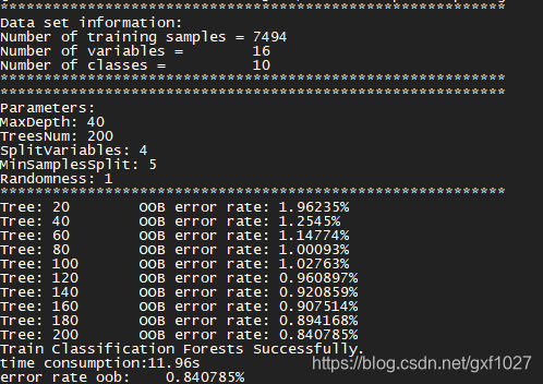
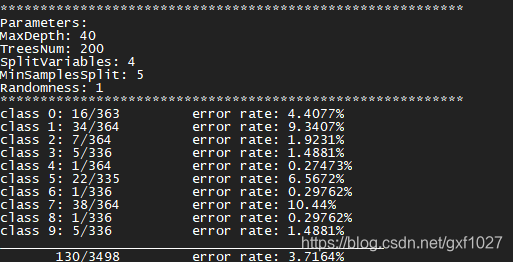
训练过程(以分类为例，pendigits数据集）

示例2：测试

./rf_test -p 0 -c rf_pendigits.xml -d ./DataSet/Classification/pendigits.tes -o test-pendigits.out

• -c: RF模型文件，即rf_train输出到本地的模型文件
• -d: 测试数据集，格式与训练集相同
• -o: 输出结果至文件

2.3.2 代码嵌入方式（推荐）

包含src目录下源文件，编写训练或者预测代码。各函数及其参数在头文件中有详细说明，容易上手。以下给出训练和预测的代码片段。

训练
从本地数据文件读入数据集进行训练，计算oob-error(oob-mse)，并保存forest到本地。
（1）分类森林

#include <cmath>
using namespace std;

#include "RandomCLoquatForests.h"
#include "UserInteraction2.h"

int main()
{
	// read training samples if necessary
	char filename[500] = "./DataSet/Classification/pendigits.tra";
	float** data = NULL;
	int* label = NULL;
	Dataset_info_C datainfo;
	InitalClassificationDataMatrixFormFile2(filename, data/*OUT*/, label/*OUT*/, datainfo/*OUT*/);
	// setting random forests parameters
	RandomCForests_info rfinfo;
	rfinfo.datainfo = datainfo;
	rfinfo.maxdepth = 40;
	rfinfo.ntrees = 500;
	rfinfo.mvariables = (int)sqrtf(datainfo.variables_num);
	rfinfo.minsamplessplit = 5;
	rfinfo.randomness = 1;
	// train forest
	LoquatCForest* loquatCForest = NULL;
	TrainRandomForestClassifier(data, label, rfinfo, loquatCForest /*OUT*/, 50);// print info every 50 trees
	float error_rate = 1.f;
	OOBErrorEstimate(data, label, loquatCForest, error_rate /*OUT*/);
	// save RF model, 0:xml, 1:plain text
	SaveRandomClassificationForestModel("Modelfile.xml", loquatCForest, 0);
	// clear the memory allocated for the entire forest
	ReleaseClassificationForest(&loquatCForest);
	// release money: data, label
	for (int i = 0; i < datainfo.samples_num; i++)
   		delete[] data[i];
	delete[] data;
	delete[] label;
	return 0;
}

（2）回归森林

#include "RandomRLoquatForests.h"
#include "UserInteraction2.h"
using namespace std;

int main()
{
	// read training samples if necessary 
    char filename[500] = "./DataSet/Regression/Housing_Data_Set-R.txt"; 
	float** data = NULL;
	float* target = NULL;
	Dataset_info_R datainfo;
	InitalRegressionDataMatrixFormFile2(filename, data /*OUT*/, target /*OUT*/, datainfo /*OUT*/);
	// setting random forests parameters
	RandomRForests_info rfinfo;
	rfinfo.datainfo = datainfo;
	rfinfo.maxdepth = 40;
	rfinfo.ntrees = 200;
	rfinfo.mvariables = (int)(datainfo.variables_num_x / 3.0 + 0.5); 
	rfinfo.minsamplessplit = 5;
	rfinfo.randomness = 1; 
	rfinfo.predictionModel=PredictionModel::constant;
	rfinfo.splitCrierion = SplitCriterion::mse;
	// train forest
	LoquatRForest* loquatRForest = NULL;
	TrainRandomForestRegressor(data, target, rfinfo, loquatRForest /*OUT*/, false, 20); // print info every 20 trees
	float* mean_squared_error = NULL;
	MSEOnOutOfBagSamples(data, target, loquatRForest, mean_squared_error /*OUT*/);
	delete[] mean_squared_error;
	// save RF model, 0:xml, 1:plain text
	SaveRandomRegressionForestModel("testModelfile-R.xml", loquatRForest, 0);
	// clear the memory
	ReleaseRegressionForest(&loquatRForest);
	// release money: data, target
	for (int i = 0; i < datainfo.samples_num; i++)
		   delete[] data[i];
	delete[] data;
	delete[] target;
	return 0;
}

说明

• 以上代码仅为主干，实际使用需对函数返回值进行判断。
• RF结构体对象loquatForest的内存由TrainRandomForestClassifier /TrainRandomForestRegressor 负责分配，由ReleaseClassificationForest /ReleaseRegressionForest 释放内存，用户无需对其分配或者释放
• OOBErrorEstimate 计算out-of-bag分类错误率，输入参数data, label必须与训练时相同,MSEOnOutOfBagSamples类同
• InitalClassificationDataMatrixFormFile2/InitalRegressionDataMatrixFormFile2 从本地文件读取数据集，文件格式与“命令行方式”中相同。也可以自行准备训练数据，就可以不调用上述函数。

预测

// 分类森林：label_index用于返回预测的类别
EvaluateOneSample(data, loquatForest, label_index /*OUT*/, 1);
// 回归森林：target_predicted用于返回预测的目标值
EvaluateOneSample(data, loquatForest, target_predicted /*OUT*/);

• 提供单个样本的分类/回归接口，对整个数据集可以循环解决。
• 分类森林的最后一个参数表示预测方式，1：hard，0：soft decision。

3. Python接口

未完待续

4. 实验

4.1 数据集

名称	分类/回归	来源	样本数	特征数	类别数
chess-krvk	classification	UCI	28056	6	18
Gisette	classification	UCI	6000/1000	5000	2
ionosphere	classification	UCI	351	34	2
mnist	classification	libsvm	60000/10000	780	10
MAGIC_Gamma_Telescope	classification	UCI	19020	10	2
pendigits	classification	UCI	7494/3498	16	10
spambase	classification	UCI	4601	57	2
Sensorless_drive_diagnosis	classification	UCI	58509	48	11
Smartphone Human Activity Recognition	classification	UCI	4242	561	6
waveform	classification	UCI	5000	40	3
satimage	classification	UCI	6435	36	6
Car Evaluation	classification	UCI	1728	6	4
sonar	classification	UCI	208	60	2
abalone	regression	UCI	4177	8	——
airfoil_self_noise	regression	UCI	1503	5	——
Bike-Sharing1	regression	UCI	17379	14	——
Combined_Cycle_Power_Plant	regression	UCI	9568	4	——
elevators	regression	openml	16599	18	——
QSAR fish toxicity	regression	UCI	908	6	——
Housing	regression	kaggle	506	13	——
Parkinsons_Telemonitoring2	regression	UCI	5875	19	——
Superconductivty	regression	UCI	21263	81	——
YearPredictionMSD	regression	Million Song Dataset/ UCI	515345	90	——

1. Bike-Sharing: 原数据集去掉第1、2列
2. Parkinsons_Telemonitoring: 预测输出(output)是2维的。将原数据集第1列（subject number）去掉，UCI网站上记录“Number of Attributes：26”但根据下载的数据集只有22维（包括2维output)

4.2 参数

        使用2.2中参数，下一小节表格中“参数”列为 [TreesNum, SplitVariables, MaxDepth, MinSamplesSplit] （randomness均为1，即经典RF）。实验并没有对参数进行调优，而是根据经验选取了个人认为比较合理的参数组合。实验目的一方面是为了验证算法实现的正确性，另一方面也想说明RF对参数敏感度较低（相比SVM）。

Clearly, some algorithms such as glmnet and svm are much more tunable than the others,
while ranger(random forest) is the algorithm with the smallest tunability.^[6]

4.3 结果

        如果没有特殊说明，分类和回归问题的实验结果分别通过out-of-bag分类错误率（%）和out-of-bag 均方误差(Mean Square Error (MSE))来统计，结果运行10次取平均和标准差。可以看到，大多数数据集都采用了默认的参数，也能达到较理想效果。

The out-of-bag (oob) error estimate
…This has proven to be unbiased in many tests^[2].

数据集	参数	oob error(%)/mse	分类/回归
chess-krvk	[500, 2*, 40, 5]	16.46636±0.07493	C
Gisette	[200, 70*, 40, 5]	2.932105±0.10090(oob) 3.010±0.13333(test set)	C
ionosphere	[200, 5*, 40, 5]	6.325±0.213	C
mnist	[200, 27*, 40, 5]	3.307166±0.02863(oob) 3.066±0.0665(test set)	C
MAGIC_Gamma_Telescope	[200, 3*, 40, 5]	11.8559±0.04347	C
pendigits	[200, 4*, 40, 5]	0.880822±0.03428(oob) 3.670668±0.049843(test set)	C
spambase	[200, 7*, 40, 5]	4.514335±0.10331	C
satimage	[500, 6*, 40, 5]	8.102018±0.057777	C
Sensorless_drive_diagnosis	[200, 6*, 40, 5]	0.169049±0.009346	C
Smartphone Human Activity Recognition	[200, 23*, 40, 5]	7.39415±0.1159	C
waveform	[500, 6*, 40, 5]	14.70493±0.19792	C
Car Evaluation	[200,2*,40,5]	1.9456±0.11923	C
sonar	[200,7*,40,2]	14.961±0.8646	C
abalone	[500, 3#, 40, 5]	4.58272±0.008826	R
airfoil_self_noise	[200, 2/5, 40, 5]	3.83345±0.034283	R
Bike-Sharing	[500, 5#, 40, 5]	29.7227±0.84333	R
Combined_Cycle_Power_Plant	[200, 2/4, 40, 5]	9.94693±0.031153	R
elevators	[200, 10/18, 40, 5]	7.1859E-06±3.15264E-08	R
QSAR fish toxicity	[200, 2#, 40, 2]	0.7669898±0.003282	R
Housing	[200, 4#, 40, 5]	10.077±0.1923	R
Parkinsons_Telemonitoring3	[200,19,40,5]	[1.437, 2.523]±[0.01706, 0.03033]	R
Superconductivty	[200, 27#, 40, 5]	81.4527±0.2781	R
YearPredictionMSD	[100, 30#, 40, 50]	83.1219±0.05236	R

*: 表示使用分类森林默认的$\sqrt{variable\_num}$作为SplitVariables参数;
#:表示使用回归森林默认的​​$\frac{variable\_num\_x}{3}$作为SplitVariables参数
3: Parkinsons_Telemonitoring的预测输出是2维的，本算法并不是把它分解为两个独立回归问题，而是直接使用多维输出数据进行训练。

5. 分析

5.1 参数影响

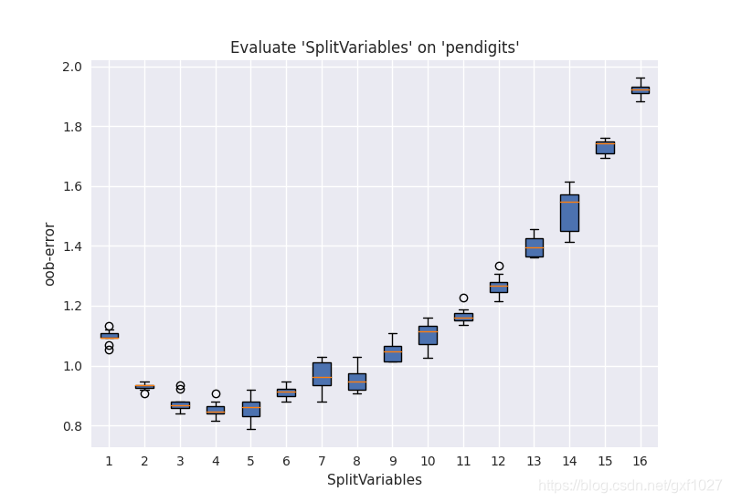
        通常RF在默认参数设定下也能取得较理想的效果，通过对参数（见2.2节）调优可以获得更佳的分类/回归效果。一般可以对TreesNum和SplitVariables进行调优。通常认为增加TreesNum会使泛化误差下降（当然也有特例）。如下图，展示了随着树增加，oob error/oob-mse呈现下降的趋势。

        SplitVariables是控制RF随机性的主要参数，当它增加时树之间的关联性也随之增加，而关联性增加会导致分类/回归误差提高^[2]。从可调性(Tunability)角度考虑，调节SplitVariables对性能提升的贡献是最大的。而SplitVariables选择默认设定时，通常也能取得不错的效果。

The correlation between any two trees in the forest. Increasing the correlation increases the forest error rate.^[2]
In ranger(random forest) mtry is the most tunable parameter which is already common knowledge and is implemented in software packages such as caret.^[6]

下图为pendigits数据集上，不同SplitVariables（样本为16维，TreesNum=500）参数下的分类oob error。

下图为mnist数据集（780维，训练：60000, 测试：10000），不同SplitVariables参数下的分类oob error和test error，训练参数为 $[TreesNum=200,MaxDepth=40,MinSamplesSplit=2]$ 。选取SplitVariables参数值为[ 1, 5, 10, 15, 20, 27, 28, 30, 35, 40, 50, 60, 80, 100, 150, 200, 250, 300, 350, 400, 450, 500, 550, 600, 650, 700]。当节点候选的分类特征数为28～50附近时分类错误率较小。

通过上面两个实验，说明SplitVariables设置成默认值$\sqrt{variable\_num}$能够取得比较理想的分类错误率。

5.2 特征重要性

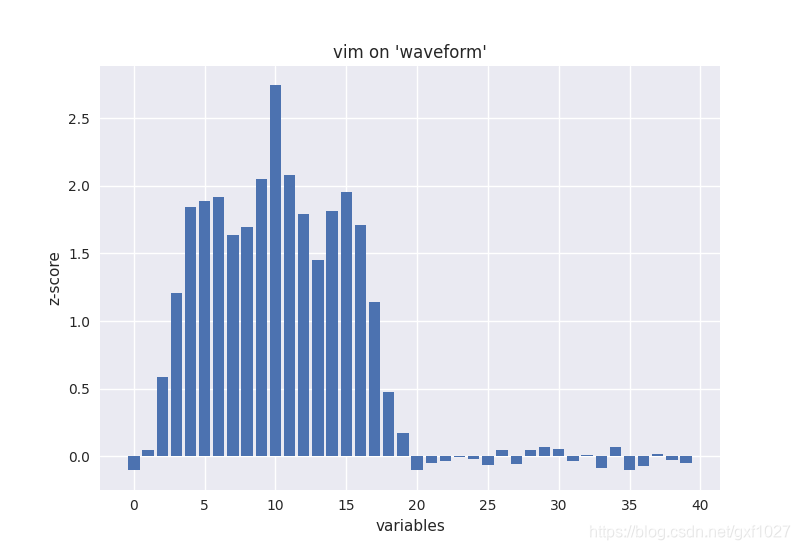
        特征重要性(variable importance)的评估是RF“自带”的一个特性。采用oob数据的特征随机交换的方法来估计特征重要性。对于数据集"waveform"，结果如下图所示，可见后一半特征的重要性几乎为0，这是因为waveform的后19维特征是随机噪声，因此variable importance计算结果符合上述情况。

5.3 Margin

Margin可以用来度量分类器对分类结果的可信程度，如果margin值很低，说明分类结果可信度不高。随机森了的margin可以这么定义^[1]：
$$mg(X,Y)=a{v}_{k}I(h_k(X)=Y)-ma{x}_{j\ne Y}a{v}_{k}I(h_k(X)=j)$$
公式含义就是样本被分到正确类别$Y$的概率—被分到其他类别$j\ne Y$的最大概率。

The margin measures the extent to which the average number of votes at X,Y for the right class exceeds the average vote for any other class. The larger the margin, the more confidence in the classification^[1].

实验使用mnist数据集，下图展示oob样本的平均margin与随机森林中树数量的关系，"概率"为样本被分为某类的oob随机树数量/所有该样本oob树数量。可以看到训练集平均margin值随着随机树数量增加而提升。

5.4 多目标回归

这里多目标指的是回归目标是多维的，一般称为multivariate regression或者multi-target regression。可以将多维目标分解为多个单独的回归问题，即可以对每一维输出输出单独训练一个模型，那么输出有$N$维就要训练$N$个随机森林模型，预测时也要获取多个随机森林的输出。使用随机森林也可以直接对多维输出（多目标）进行训练，这里也使用这种方法对多维输出进行预测。
使用Tetuan-City-power-consumption数据集来进行试验，原始数据集是通过时间、温度、湿度、风速等6个变量来预测城市3个配电网的能源消耗，即输入6维，输出3维。由于“时间”变量难以使用，所以分解为[minute,hour,day,month,weekday,weekofyear] 6个变量，加上原始的5个气象变量，形成新的11维输入。RF参数为[200, 3^#, 60, 2]（参数含义见4.2节）。由于输出具有明确物理含义，且都是正数，衡量回归准备度的指标不再使用oob-mse，而是使用oob样本的平均偏离度$\frac{|t_{predict}-t|}{t}$。下图反映了当RF中随机树数量增加时，三个输出维度的平均偏离度变化。可以看到随着随机树增加，偏离度呈下降趋势，基本都在200颗树时达到<1.8%的回归准确度。

5.5 随机程度

在每个节点分裂时可选三种随机性，在"2.2.2 关于节点分裂方式"小节中已经有详细说明。
根据实验，并没有发现选择哪种随机性能明显优于其它选择，也没有证据证明哪种随机性在大多数数据集上呈现一致的优势。以下展示两个数据集上三种随机性oob-error和oob-mse与随机树的关系。

有关上图的一些说明：

1. 参数1–week：传统的随机森林算法;
   参数2–moderate：在特征（变量）最大值与最小值之间平均划分N个切分点的方法;
   参数3–extreme：extremely randomized trees方法，在特征（变量）最大值与最小值范围内随机选取切分值。

在mnist数据集上使用三种分裂随机方法，RF模型中每棵随机树的平均深度、节点数量和叶子节点数量见下表。可见随着随机性增加，深度和节点数量也随之增加，符合预期。

节点分裂方法	平均深度	平均/最大节点数	平均/最大叶子节点数
week	28.8	8050.1/8545	4025.6/4273
moderate	28.9	8153.8/8619	4077.4/4310
extreme	31.7	11982.1/12859	5991.5/6430

6. 性能

        训练的速度（耗时）是算法性能的重要指标，为验证本算法的训练性能表现，在典型数据集上，对比了本算法与RTrees（opencv的随机森林实现）的训练耗时。OpenCV的RTrees使用C++实现，提供python接口，以下实验中两种算法的参数尽量保持一致。

实验结果

所有实验都运行5次取平均数，OpenCV版本为4.1.2，需要说明的是：RTrees最大深度(MaxDepth)的最大值为25。实验环境：win64，CPU：3.7GHz，内存：12G。实验参数如下表。

数据集	OpenCV-RF	本文RF-D40	本文RF-D25
mnist	[200, 27*, 25, 5]	[200, 27*, 40, 5]	[200, 27*, 25, 5]
spambase	[200, 7*, 25, 5]	[200, 7*, 40, 5]	[200, 7*, 25, 5]

mnist数据集上的运行结果

mnist	OpenCV-RF	本文RF-D40	本文RF-D25
耗时(s)	207.12	213.90	213.92
平均深度/树	–	29.6	25
平均节点数/树	–	8060	8032

spambase数据集上的运行结果

spambase	OpenCV-RF	本文RF-D40	本文RF-D25
耗时(s)	2.69	1.87	1.71
平均深度/树	–	32.5	25
平均节点数/树	–	569.5	531

从实验结果看，本文算法的训练速度基本接近RTrees，验证了本算法在实现上基本接近了常用开源代码的水平。令人不解的一点是，在mnist数据集上，RF-D25并没有因为树的深度减少而使训练耗时减少，从节点数来看D25平均每棵树的节点要比D40少30个节点左右，可能是因为到达最后几层树节点的样本实际非常少，所以在它们上的分裂计算量少到忽略不计了。

附：opencv训练RTrees的python代码核心片段（以mnist数据集为例）

import cv2
import numpy as np
......
# 读取数据集，X：样本，Y：类别
......
rf=cv2.ml.RTrees_create()
rf.setActiveVarCount(27)
rf.setMinSampleCount(5)
rf.setMaxDepth(40) # RTrees的最大深度的最大值为25，这里设置为40，而实际上用于训练的参数为25
rf.setTermCriteria((1,200,0.0))
X=X.astype(np.float32)
Y=Y.astype(np.int32)
traindata=cv2.ml.TrainData_create(X,cv2.ml.ROW_SAMPLE,Y)
rf.train(traindata)  # 对trian进行计时

参考文献

[1]. Breiman, L. Random Forests . Machine Learning 45, 5–32, 2001.

[2]. Leo Breiman, Adele Cutler. Random Forest Homepage on berkeley website.

[3]. Antonio Criminisi, Ender Konukoglu, Jamie Shotton. Decision Forests for Classification, Regression, Density Estimation, Manifold Learning and Semi-Supervised Learning. MSR-TR-2011-114, 2011.

[4]. P. Geurts, D. Ernst, and L. Wehenkel. Extremely randomized trees . Machine Learning, 63(1), 2006: 3-42.

[5]. Manuel Fernández-Delgado, Eva Cernadas, Senén Barro, Dinani Amorim. Do we Need Hundreds of Classifiers to Solve Real World Classification Problems? Journal of Machine Learning Research, 15(90):3133−3181, 2014.

[6]. Philipp Probst, Anne-Laure Boulesteix, Bernd Bischl. Tunability: Importance of Hyperparameters of Machine Learning Algorithms. Journal of Machine Learning Research, 20(53):1−32, 2019.

[7]. Gilles Louppe. Understanding Random Forests: From Theory to Practice. PhD thesis, 2014, arXiv:1407.7502.