Tutorial on Binary Descriptors – part 1(转)

Tutorial on Binary Descriptors – part 1

Why Binary Descriptors?

Following the previous post on descriptors, we’re now familiar with histogram of gradients (HOG) based patch descriptors. SIFT[1], SURF[2] and GLOH[3] have been around since 1999 and been used successfully in various applications, including image alignment, 3D reconstruction and object recognition. On the practicle side, OpenCV includes implementations of SIFT and SURF and Matlab packages are also available (check vlfeat for SIFT and extractFeatures in Matlab computer vision toolbox for SURF).

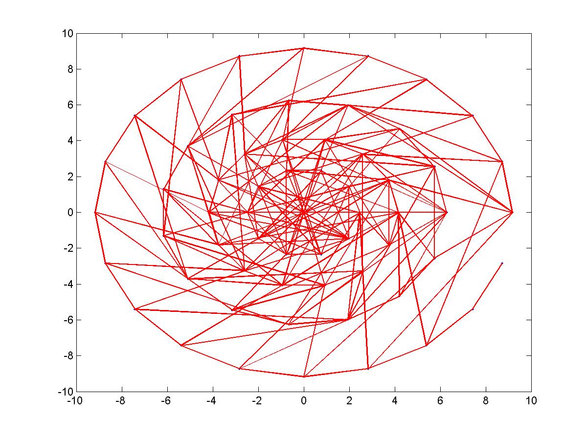
BRISK descriptor – sampling pairs

So, if there no question about SIFT and SURF performance, why not use them in every application?

 

Remember that SIFT and SURF are based on histograms of gradients. That is, the gradients of each pixel in the patch need to be computed. These computations cost time. Even though SURF speeds up the computation using integral imags, this still isn’t fast enough for some applications. Also, SIFT and SURF are patent-protected (that’s why they’re named “nonfree” in OpenCV ).

This is where binary descriptors come in handy. Imagine one can encode most of the information of a patch as a binary string using only comparison of intensity images. This can be done very fast, as only intensity comparisons need to be made. Also, if we use the hamming distance as a distance measure between two binary strings, then matching between two patch descriptions can be done using a single instruction, as the hamming distance equals the sum of the XOR operation between the two binary strings. This is exactly the common line and rational behind binary descriptors.

In the following series of posts I’ll explain all one needs to know on binary descriptors, covering BRIEF[4], ORB[5], BRISK[6] and FREAK[7], including some examples of OpenCV usage and performance comaprison.But first, let’s lay the common grounds by giving a short introduction, explaining the commonalities of the family of binary descriptors.

Introduction to Binary Descriptors

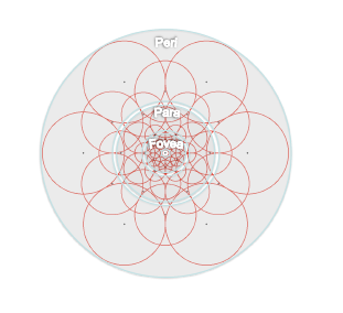
In general, Binary descriptors are composed of three parts: A sampling pattern, orientation compensation and sampling pairs. Consider a small patch centered around a keypoint. We’d like to describe it as a binary string. First thing, take a sampling pattern around the keypoint, for example – points spread on a set of concentric circles. Below you can look at BRISK’s (left) and FREAK’s (right) sampling pattern.

BRISK descriptor – sampling pattern

FREAK descriptor – sampling pattern

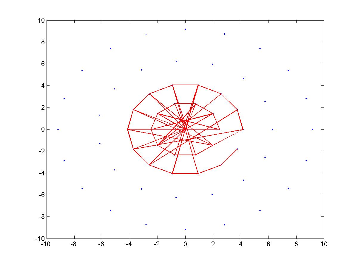
Next, choose, say, 512 pairs of points on this sampling pattern. Now go over all the pairs and compare the intensity value of the first point in the pair with the intensity value of the second point in the pair – If the first value is larger then the second, write ‘1’ in the string, otherwise write ‘0’. That’s it. After going over all 512 pairs, we’ll have a 512 characters string, composed out of ‘1’ and ‘0’ that encoded the local information around the keypoint. In the first figure of the post is BRISK’s pairs and  Below you can take a look at FREAKS’s pairs:

FREAK descriptor – sampling pairs

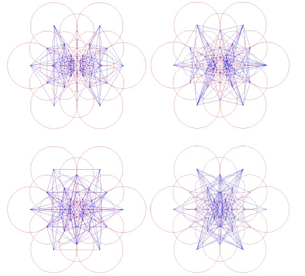
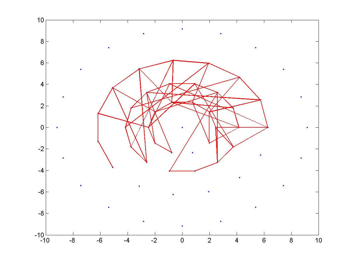
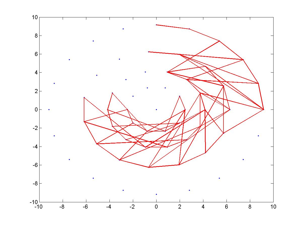
And here are five figures presenting BRISK’s pairs again, where each figure presented only 100 pairs:

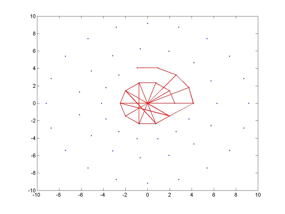
BRISK descriptor – sampling pairs

BRISK descriptor – sampling pairs

BRISK descriptor – sampling pairs

BRISK descriptor – sampling pairs

 

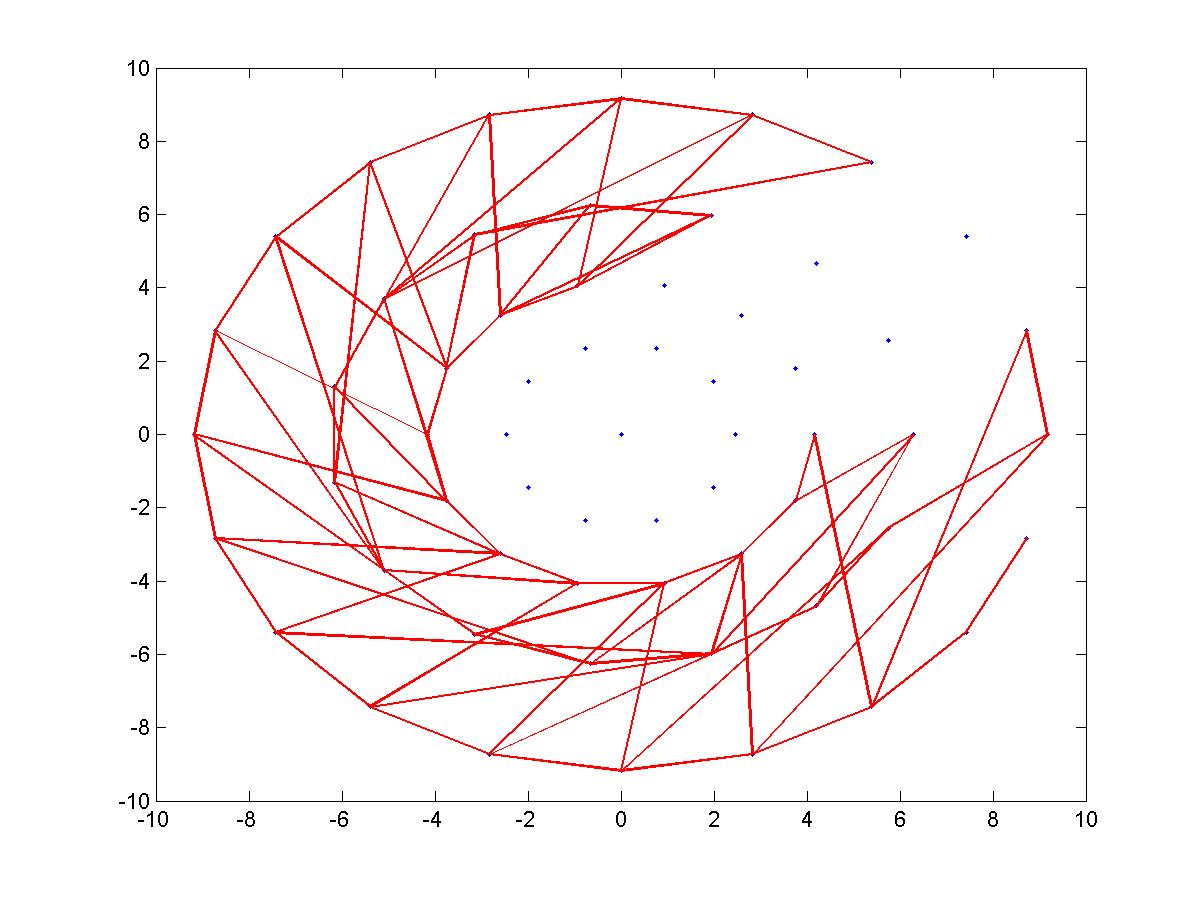
BRISK descriptor – sampling pairs

What about matching? Given two keypoint, first apply the above procedure on both of them, using of course, the same sampling pattern and the same sequence of pairs. Once will have two binary string, comparing them is easy (and fast) – just count the number of bits where the strings diff, or equivalently apply sum(xor(string1,string2)).

You probably noticed I skipped the second part of orientation compensation; just wanted to explain the basics before we elaborated on the use of orientation. Well, suppose we take a patch and describe it as a binary string using the procedure explained above. Now we rotate the patch by some theta and again extract a binary string describing the rotated patch. Will both description strings be similar? Probably not, as the pattern rotated, but the pairs remained the same.Orientation compensation is a phase where the orientation angle of the patch is measured and the pairs are rotated by that angle to ensure that the description is rotation invariant.

Every binary descriptor has its own sampling pattern, own method of orientation calculation and its own set of sampling pairs. I’ll conclude this post with a table comparing all the binary descriptors in those respects. I know these are all buzzwords , but in the following posts I will talk about every descriptor in detail, and hopefully, everything will become clear.

	Sampling pattern	Orientation calculation	Sampling pairs
BRIEF	None.	None.	Random.
ORB	None.	Moments.	Learned pairs.
BRISK	Concentric circles with more points on outer rings.	Comparing gradients of long pairs.	Using only short pairs.
FREAK	Overlapping Concentric circles with more points on inner rings.	Comparing gradients of preselected 45 pairs.	Learned pairs.

Hope to see you in the part 2 of this tutorial which will cover the BRIEF descriptor.

Gil.

References:

[1] Lowe, David G. “Object recognition from local scale-invariant features.”Computer vision, 1999. The proceedings of the seventh IEEE international conference on. Vol. 2. Ieee, 1999.‏

[2] Bay, Herbert, Tinne Tuytelaars, and Luc Van Gool. “Surf: Speeded up robust features.” Computer Vision–ECCV 2006. Springer Berlin Heidelberg, 2006. 404-417.‏

[3] Mikolajczyk, Krystian, and Cordelia Schmid. “A performance evaluation of local descriptors.” Pattern Analysis and Machine Intelligence, IEEE Transactions on27.10 (2005): 1615-1630.‏

[4] Calonder, Michael, et al. “Brief: Binary robust independent elementary features.” Computer Vision–ECCV 2010. Springer Berlin Heidelberg, 2010. 778-792.‏

[5] Rublee, Ethan, et al. “ORB: an efficient alternative to SIFT or SURF.” Computer Vision (ICCV), 2011 IEEE International Conference on. IEEE, 2011.‏

[6] Leutenegger, Stefan, Margarita Chli, and Roland Y. Siegwart. “BRISK: Binary robust invariant scalable keypoints.” Computer Vision (ICCV), 2011 IEEE International Conference on. IEEE, 2011.‏

[7] Alahi, Alexandre, Raphael Ortiz, and Pierre Vandergheynst. “Freak: Fast retina keypoint.” Computer Vision and Pattern Recognition (CVPR), 2012 IEEE Conference on. IEEE, 2012.‏

原文链接：https://gilscvblog.com/2013/08/26/tutorial-on-binary-descriptors-part-1/