图像处理的变分法研究（1）——11月第一阶段进展报告

最新推荐文章于 2024-04-22 10:11:23 发布

_helen_520

最新推荐文章于 2024-04-22 10:11:23 发布

阅读量3.9k

点赞数 3

分类专栏：盲解卷积硕士课题文章标签：图像处理变分迭代法

本文链接：https://blog.csdn.net/haronchou/article/details/78478584

版权

盲解卷积硕士课题专栏收录该内容

4 篇文章 3 订阅

订阅专栏

按：10.30——11.8（共10天）阶段性报告（开题答辩后一个星期）这部分的笔记看纸质的比较好，总结的较好些。

一、总变分的物理数学背景

参考资料：（1）Gilboa的课程Variational Methods in Image Processing. Course Website 主要是notes1—notes5, exercise1 & exercise2(TVBD部分)
(2)冯象初《图像处理的变分和偏微分方程》chap1 & chap2
(3)Gilboa推荐的数学书籍《Mathematical Problems in Image Processing:Partial Differential Equations and the Calculus of Variations》图像处理中的数学问题chap2 & chap3
(4)PPT 《数学物理方程》学生群里下载的国科大的，关于变分法那一章。另外配套的教材里也有变分法一章，有一些基本推导，可以加强理解。

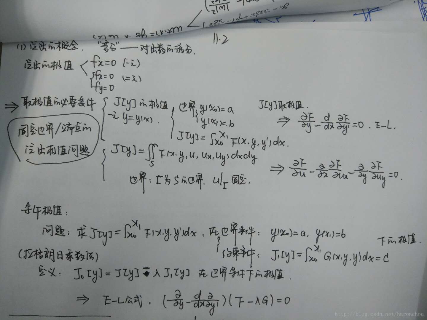
泛函的概念、泛函极值

变分——就是泛函J对函数u的微分。泛函——自变量是函数，因变量是一个值，达到一一对应。泛函极值——求一个最佳的函数使得因变量取最大值。因此，对J(u)泛函求极值，要对J(u)求微分（二元时求偏导），就是变分了。
——可以推导，无论一元还是二元，minJ(u)当满足E-L公式时，取得极值。得到E-L公式后，就是求解这个公式，方法是用时间演化，即ut = E-L = 0. 其中dt的取值有限制，要满足CFL条件。

$微信图片_20171108115242](C:\Users\Haron\Desktop\Typora Files\微信图片_20171108115242.jpg)![这里写图片描述$

物理学上的泛函

三类典型的数学物理方程都是偏微分方程。边界条件+初始条件才能确定解。

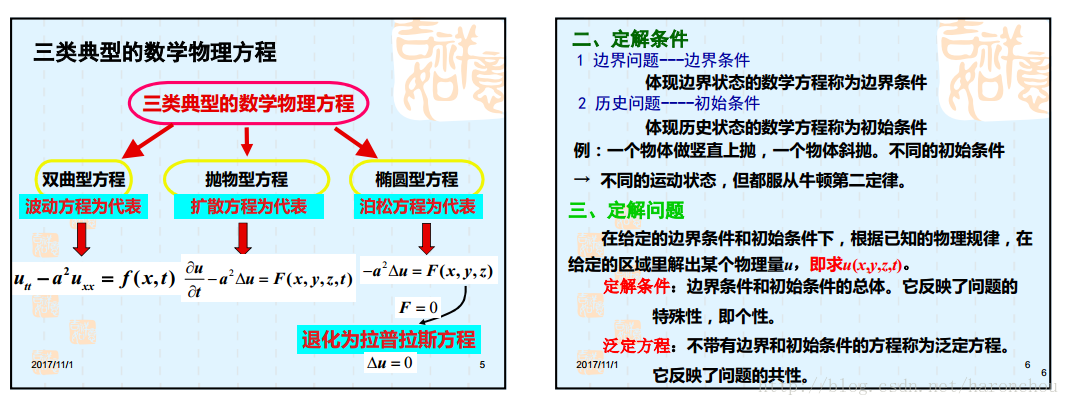
$PPT](C:\Users\Haron\Desktop\Typora Files\PPT.PNG)![这里写图片描述$

其中，我们的扩散方程与我们图像处理息息相关。
在冯象初《书》中，我们可以总结：div(c gradu)=0是线性扩散，系数为常数。c = 1时的扩散方程，ut = gradu。这个方程的解 == 用高斯函数与U卷积表示。其中高斯函数: $\sigma = \sqrt{2t}$ 。这一证明可见matlab代码：haron_LinearDiffusion.m 确实线性扩散收敛后的结果与高斯卷积模糊的结果是一样的。（代码1，贴图）。

$u_t = \Delta{u} = u_{xx}+u_{yy}$ 线性扩散: $div(c\times u(x))$ ，其中 $c =1$ , $u^{n+1} = u^n+dt\times(\Delta u)$ .
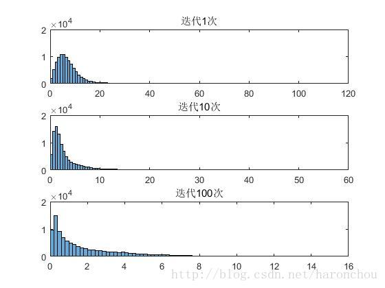
其中，根据迭代过程的收敛性看，100次已经达到了稳定。

$线性扩散(laplace算子)](C:\Users\Haron\Desktop\Typora Files\线性扩散(laplace算子).jpg)![这里写图片描述$

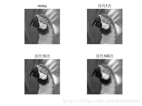
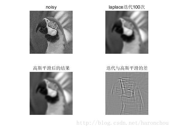
由于线性扩散与高斯卷积等价，可以看出经历相同时间t后，线性扩散收敛后的结果与高斯平滑的结果一致，它们的差如第四张图。

$线性扩散与高斯卷积](C:\Users\Haron\Desktop\Typora Files\线性扩散与高斯卷积.jpg)![这里写图片描述$

这个是线性扩散迭代后的估计图像的直方图分布，可以看出随着迭代的进行，直方图越来越平坦，意味着图像被平滑掉了。

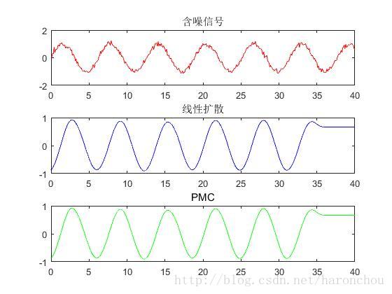
$直方图](C:\Users\Haron\Desktop\Typora Files\直方图.jpg)![这里写图片描述$

一维信号用线性扩散和PMC去噪的结果，两者类似（其中高斯噪声标准差为10）。注意：这里dt时间步长的选择对迭代次数有关，PMC中K值的选择跟噪声标准差有关。目前只能手动选择看效果，如何设计算法自动选择最佳的参数值有待研究。

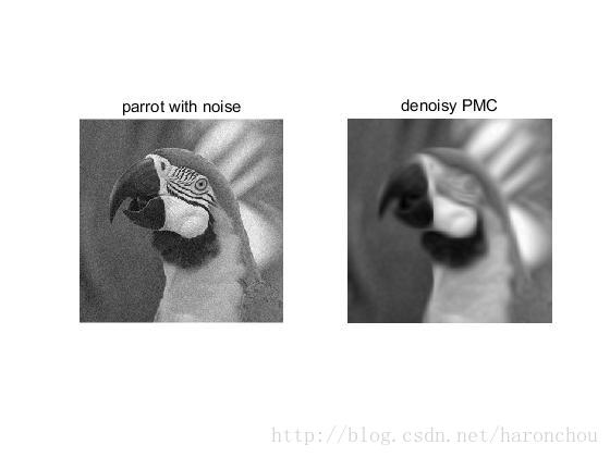
$线性扩散与PMC去噪](C:\Users\Haron\Desktop\Typora Files\线性扩散与PMC去噪.jpg)![这里写图片描述$

这里是PMC用在二维图像上的效果。
$二维PMC](C:\Users\Haron\Desktop\Typora Files\二维PMC.jpg)![这里写图片描述$

那么，下面我们要做的是：根据方法的不同，我们设计了不同的泛函（能量泛函），求出相应的E-L公式。最后我们需要求解E-L方程。人们还设计了不同的求解方法去求解E-L。也有不同的方法去离散E-L方程，如：有限元法、有限差分、？（忘了）等。

下一步工作计划：找出有哪些不同的泛函（对应的物理解释）、相应的E-L方程、如何求解E-L？最后Matlab实现这些方法、采用一定的评价指标评价这些方法、总结优缺点、找到自己的突破点！

这些计划的信息来源：历年博硕士论文（优秀的）——为了得到关于其基本理论的阐述：如变分法的发展（哪些人做了哪些修改、效果、基本原理、他们的英文文章来源等）。

自我总结与评价

这段时间的工作非常基础，但是似乎与主要工作方向偏离了。看了很多资料（英文），看了很多理论，写了很多笔记，写了一点点代码(这部分基础代码还是对理解有帮助的！)。还没有得到我最想要的东西，最想看的最想总结的，接下来的半个月要加油！

代码1 比较线性扩散和高斯卷积

%%
%要求1：作为时间的函数，计算和绘制下列度量的图
%               （1）标准偏差
%               （2）时间t在0.1,1,10时， 图像的梯度幅度值的三个直方图。
%       解释其趋势及发生原因
%要求2：将扩散与等效sigma的高斯卷积相比较。如有差异解释原因
%%结论： 扩散与高斯卷积的结果大致相同，略微差别。
%%
f_parrot = imread('parrot.png');
f_parrot = double(rgb2gray(f_parrot));
% imshow(f_girl,[0,255]), title('Original girl image');
%加噪声
N_std = 10; % noise standard deviation
noise = randn(size(f_parrot))*N_std;
f = f_parrot + noise;
% figure(2); imshow(f,[0,255]), title('Sun-girl with noise');
C = 1;
%%
%画t=0.1,1,10处的梯度值的直方图
dt = 0.1;
Iter1 =1;
u1 = diffusion_lin(f,C, Iter1, dt);
grad1 = gradF(u1);
u2 = diffusion_lin(f,C, Iter1*10, dt);
grad2 = gradF(u2);
[u3, J3] = diffusion_lin(f,C, Iter1*100, dt);
grad3 = gradF(u3);
%画图显示
figure(1);
t = 0:0.01:10;
plot(t, sqrt(2*C*t),'r');legend('sqrt(2*C*t)');xlabel('t'), ylabel('\sigma(t)');
figure(2);
subplot(221);imshow(f,[]),title('noisy');
subplot(222);imshow(u1,[]),title('迭代1次');
subplot(223);imshow(u2,[]),title('迭代10次');
subplot(224);imshow(u3,[]),title('迭代100次');
figure(3);
subplot(311); histogram(grad1);title('迭代1次');
subplot(312);histogram(grad2);title('迭代10次');
subplot(313); histogram(grad3);title('迭代100次');
%%
figure(4);
plot(1:100, J3, 'b');
%%
%%高斯核卷积对比
n = 100;
t = n * dt;
gauss = fspecial('gaussian',size(f),sqrt(2*t));
u_gaussian = imfilter(f, gauss, 'symmetric');
figure(5);
imshow(u_gaussian,[]), title('高斯平滑后的结果');
u_difference = u3 - u_gaussian;
figure(6); imshow(u_difference,[]),
title('迭代与高斯平滑的差');
%%
function grad_f = gradF(f)
[nx ny] = size(f);
f_x = (f(:,[2:nx nx])-f(:,[1 1:nx-1]))/2;
f_y = (f([2:ny ny],:)-f([1 1:ny-1],:))/2; 
grad_f = (sqrt(f_x.^2+f_y.^2));
end

%%
function [u, J]=diffusion_lin(f,C,Iter,dt)
% u=diffusion_lin(f,C,Iter,dt)  线性扩散 Sun-girl 图像
% parameters:
% f      = input image (2D gray-level)
% C      = constant diffusion coefficient
% Iter   = number of iterations 
% dt     = time step 
I = f;%读入图像
[nx ny] = size(f);
for i = 1: Iter
     Iold = I;
     I_xx = I(:,[2:nx nx])+I(:,[1 1:nx-1])-2*I;%二阶微分
     I_yy = I([2:ny ny],:)+I([1 1:ny-1],:)-2*I;
     I_t = C * (I_xx + I_yy);
     I = I + dt* I_t;
     Inew = I;
     J(i) = norm(Iold - Inew);
end
u = I;
end

%%part1：一维降噪，线性和PMC
t = 0:0.1:40;
y_true = sin(t);
%加噪声
N_std = 0.1; % noise standard deviation
noise = randn(size(y_true))*N_std;
y = y_true + noise;
subplot(311);plot(t,y,'r');title('含噪信号')
%%线性扩散
dt = 0.5;%[0,1]之间
Iter = 100;
[u1, J1] = diffusion_lin1D(y, 1, Iter, dt);
subplot(312);plot(t,u1,'b');title('线性扩散');
K = 2;
[u2, J2] = diffusion_PMC(y, K, Iter, dt);
subplot(313);plot(t,u2,'g');title('PMC');
figure;plot(1:Iter, J1,'b');hold on;plot(1:Iter, J2,'r');legend('Linear','PMC')
function [u, J] = diffusion_PMC(f,K,Iter,dt)
%公式推导见Exercise1
[nx ny] = size(f);
for i = 1: Iter
    fold = f;
    f_xx = f([2:ny ny])+f([1:ny-1 ny-1]) -2*f;
    f_x = (f([2:ny ny]) - f([1:ny-1 ny-1])) / 2;
    temp = ((f_x ./ K).^2 + 1 ) .^1.5;
    f_t = f_xx ./ temp;
    fnew = fold + dt.* f_t;
    f = fnew;
    J(i) =norm(fold - fnew);
end
   u = f;
end

function [u, J]=diffusion_lin1D(f,C,Iter,dt)
% u=diffusion_lin(f,C,Iter,dt)  线性扩散 Sun-girl 图像
% parameters:
% f      = input image (2D gray-level)
% C      = constant diffusion coefficient
% Iter   = number of iterations 
% dt     = time step 
I = f;%读入图像
[nx ny] = size(f);
for i = 1: Iter
     Iold = I;
     I_xx = I([2:ny ny])+I([1:ny-1 ny-1]) -2*I;%二阶微分
     I_t = C * (I_xx);
     I = I + dt* I_t;
     Inew = I;
     J(i) = norm(Iold - Inew);
end
u = I;
end

close all, clc;
f_parrot = imread('parrot.png');
f_parrot = double(rgb2gray(f_parrot));
% imshow(f_girl,[0,255]), title('Original girl image');
%加噪声
N_std = 10; % noise standard deviation
noise = randn(size(f_parrot))*N_std;
f = f_parrot + noise;
% figure(2); imshow(f,[0,255]), title('parrot with noise');
K =10;
Iter = 100;
dt = 0.01;
[u1, J1] = diffusion_PMC(f, K, Iter, dt);
subplot(121),imshow(f,[]),title('parrot with noise');
subplot(122),imshow(u1,[]),title('denoisy PMC');
figure;plot(1:Iter, J1);
%PMC降噪
function [u, J] = diffusion_PMC(f,K,Iter,dt)
%公式推导见Exercise1
[nx ny] = size(f);
for i = 1: Iter
    fold = f;
     f_x = (f(:,[2:nx nx])-f(:,[1 1:nx-1]))/2;
    f_y = (f([2:ny ny],:)-f([1 1:ny-1],:))/2;
    f_xx = f(:,[2:nx nx])+f(:,[1 1:nx-1])-2*f;
    f_yy = f([2:ny ny],:)+f([1 1:ny-1],:)-2*f;
    A = (1 + (f_x.^2 + f_y.^2)./ K.^2) .^1.5;
    temp = (1 + f_x .^2) .* f_yy + (1 + f_y .^2) .* f_xx;
    f_t = temp ./ A;
    fnew = fold + dt.* f_t;
    f = fnew;
    J(i) =norm(fold - fnew);
end
   u = f;
end

_helen_520

关注

3
点赞
踩
22

收藏

觉得还不错? 一键收藏
3
评论
图像处理的变分法研究（1）——11月第一阶段进展报告

按：10.30——11.8（共10天）阶段性报告（开题答辩后一个星期）这部分的笔记看纸质的比较好，总结的较好些。一、总变分的物理数学背景参考资料：（1）Gilboa的课程Variational Methods in Image Processing. Course Website 主要是notes1—notes5, exercise1 & exercise2(TVBD部分) (2)冯象初《图像处理
复制链接

扫一扫