


目录
3.python中的向量化实验(C1_W2_Lab01_Python_Numpy_Vectorization_Soln)
3.多特征线性回归模型实验(C1_W2_Lab02_Multiple_Variable_Soln)
(5).将上面步骤(3)(4)实现的代码代入梯度下降算法的上面公式(5)中
看本文前请先阅读专栏内容:“三、梯度下降法”,前文链接如下
一、问题背景
房屋价格并不是一个变量决定的,而是由多个因素共同作用决定的

二、多特征(n个特征)变量的线性回归表示方法
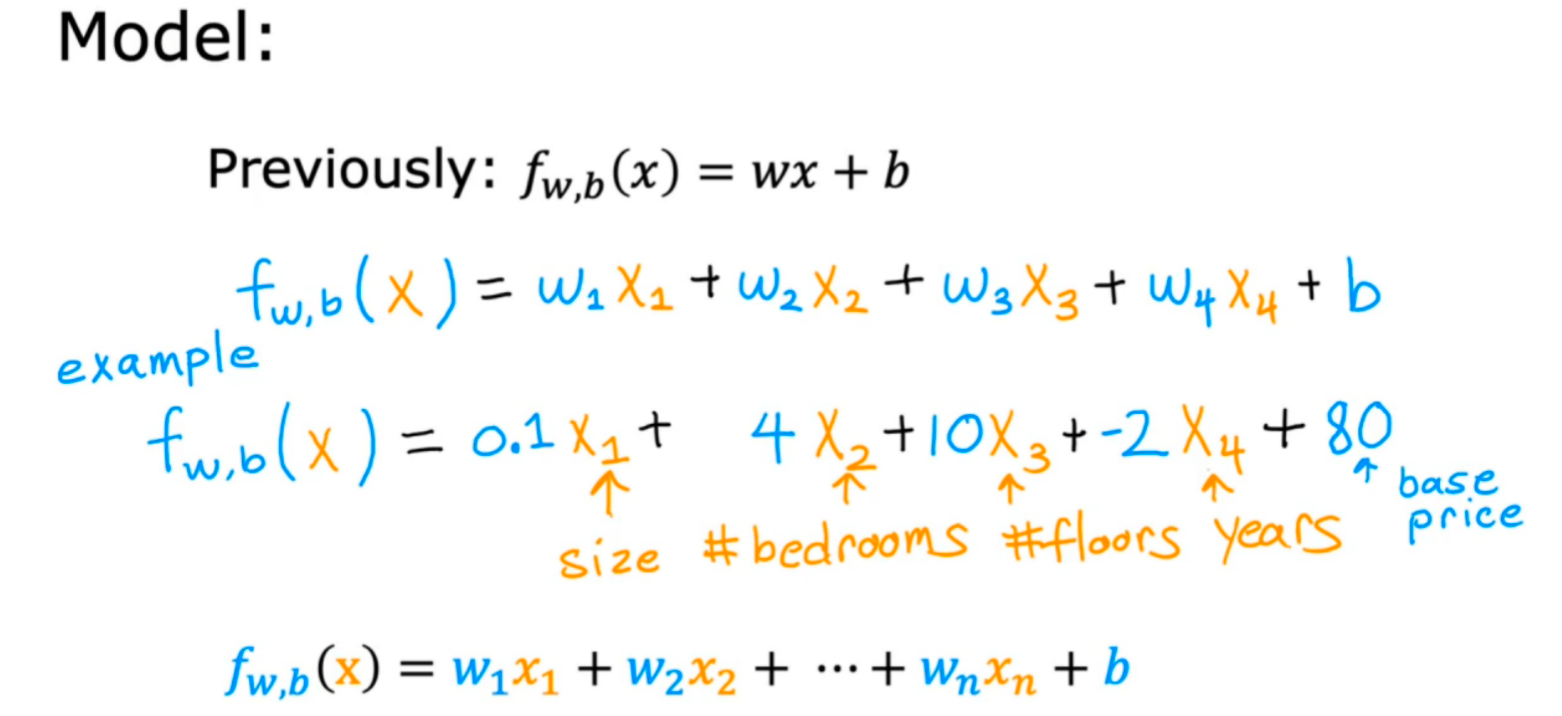

三、向量化
在python中如何表示并计算多特征线性回归模型(使用numpy工具包)

1.向量表示
# 向量表示
w = np.array([1.0,2.5,-3.3])
b = 4
x = np.array([10,20,30])
在python中数组下标是从0开始的,也就是向量w中的w1在向量中用w[0]表示。
2.两种计算方式(第二种效率更高)
# 一般计算方式fw,b(x)
f = 0
for j in range(0,n):
    f = f + w[j] * x[j]
f = f + b
# 其中 range(0,n) -> j = 0,1,2,…,n-1
# 直接用numpy库dot点乘函数计算fw,b(x)
f = np.dot(w,x) + b3.python中的向量化实验(C1_W2_Lab01_Python_Numpy_Vectorization_Soln)
(1)向量创建的各种示例
# NumPy routines which allocate memory and fill arrays with value
a = np.zeros(4);                print(f"np.zeros(4) :   a = {a}, a shape = {a.shape}, a data type = {a.dtype}")
a = np.zeros((4,));             print(f"np.zeros(4,) :  a = {a}, a shape = {a.shape}, a data type = {a.dtype}")
a = np.random.random_sample(4); print(f"np.random.random_sample(4): a = {a}, a shape = {a.shape}, a data type = {a.dtype}")![]()
其中a.shape表示a的维度,(4,) 表示有4个元素的一维向量
# NumPy routines which allocate memory and fill arrays with value but do not accept shape as input argument
a = np.arange(4.);              print(f"np.arange(4.):     a = {a}, a shape = {a.shape}, a data type = {a.dtype}")
a = np.random.rand(4); print(f"np.random.rand(4): a = {a}, a shape = {a.shape}, a data type = {a.dtype}")![]()
也可以手动指定元素:
# NumPy routines which allocate memory and fill with user specified values
a = np.array([5,4,3,2]);  print(f"np.array([5,4,3,2]):  a = {a},     a shape = {a.shape}, a data type = {a.dtype}")
a = np.array([5.,4,3,2]); print(f"np.array([5.,4,3,2]): a = {a}, a shape = {a.shape}, a data type = {a.dtype}")![]()
(2)向量操作
①索引
#vector indexing operations on 1-D vectors
a = np.arange(10)
print(a)


#access an element
print(f"a[2].shape: {a[2].shape} a[2]  = {a[2]}, Accessing an element returns a scalar")


# access the last element, negative indexes count from the end
print(f"a[-1] = {a[-1]}")


#indexs must be within the range of the vector or they will produce and error
try:
    c = a[10]
except Exception as e:
    print("The error message you'll see is:")
    print(e)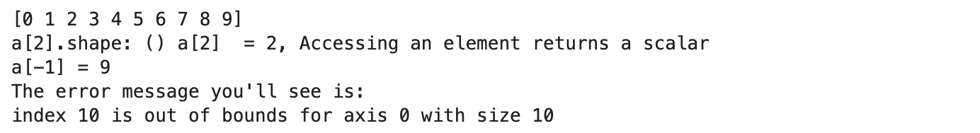
②切片Slicing
#vector slicing operations
a = np.arange(10)
print(f"a         = {a}")

#access 5 consecutive elements (start:stop:step)
c = a[2:7:1];     print("a[2:7:1] = ", c)

# access 3 elements separated by two
c = a[2:7:2];     print("a[2:7:2] = ", c)

# access all elements index 3 and above
c = a[3:];        print("a[3:]    = ", c)

# access all elements below index 3
c = a[:3];        print("a[:3]    = ", c)

# access all elements
c = a[:];         print("a[:]     = ", c)
③对向量进行符号运算
a = np.array([1,2,3,4])
print(f"a             : {a}")
# negate elements of a
b = -a
print(f"b = -a        : {b}")

# sum all elements of a, returns a scalar
b = np.sum(a)
print(f"b = np.sum(a) : {b}")

b = np.mean(a)
print(f"b = np.mean(a): {b}")

b = a**2
print(f"b = a**2      : {b}")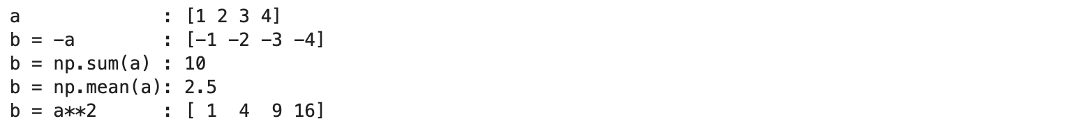
④对两个向量进行加减操作
# 相同size可以正常执行
a = np.array([ 1, 2, 3, 4])
b = np.array([-1,-2, 3, 4])
print(f"Binary operators work element wise: {a + b}")![]()
# 不同size不能正常执行,报告错误
#try a mismatched vector operation
c = np.array([1, 2])
try:
    d = a + c
except Exception as e:
    print("The error message you'll see is:")
print(e)![]()
⑤标量和向量的运算
a = np.array([1, 2, 3, 4])

# multiply a by a scalar
b = 5 * a
print(f"b = 5 * a : {b}")![]()
⑥向量之间的点积运算

# test 1-D
a = np.array([1, 2, 3, 4])
b = np.array([-1, 4, 3, 2])
c = np.dot(a, b)
print(f"NumPy 1-D np.dot(a, b) = {c}, np.dot(a, b).shape = {c.shape} ")
c = np.dot(b, a)
print(f"NumPy 1-D np.dot(b, a) = {c}, np.dot(a, b).shape = {c.shape} ")![]()
⑦ 比较 自己实现和numpy库实现的点积计算速度
#自己实现的点积计算
def my_dot(a, b):
    """
   Compute the dot product of two vectors
    Args:
      a (ndarray (n,)):  input vector
      b (ndarray (n,)):  input vector with same dimension as a

    Returns:
      x (scalar):
    """
    x=0
    for i in range(a.shape[0]):
        x = x + a[i] * b[i]
    return x
上面函数和numpy.dot()比较:
np.random.seed(1)
a = np.random.rand(10000000)  # very large arrays
b = np.random.rand(10000000)

tic = time.time()  # capture start time
c = np.dot(a, b)
toc = time.time()  # capture end time

print(f"np.dot(a, b) =  {c:.4f}")
print(f"Vectorized version duration: {1000*(toc-tic):.4f} ms ")

tic = time.time()  # capture start time
c = my_dot(a,b)
toc = time.time()  # capture end time

print(f"my_dot(a, b) =  {c:.4f}")
print(f"loop version duration: {1000*(toc-tic):.4f} ms ")

del(a);del(b)  #remove these big arrays from memory
可以看到numpy计算效率高很多,这是因为NumPy更好地利用了底层硬件的数据并行性。GPU和现代CPU实现了单指令多数据(SIMD)管道,允许并行发出多个操作。这在机器学习中至关重要,因为数据集通常非常大。
(3)矩阵的创建
a = np.zeros((3, 5))
print(f"a shape = {a.shape}, a = \n{a}")
a = np.zeros((2, 1))
print(f"a shape = {a.shape}, a = {a}")
a = np.random.random_sample((1, 1))
print(f"a shape = {a.shape}, a = {a}")
也可以手动指定矩阵元素
# NumPy routines which allocate memory and fill with user specified values
a = np.array([[5], [4], [3]]);   print(f" a shape = {a.shape}, np.array: a = \n{a}")
a = np.array([[5],   # One can also
              [4],   # separate values
              [3]]); #into separate rows
print(f" a shape = {a.shape}, np.array: a = \n{a}")
(4)矩阵操作
①索引[row, column]定位
#vector indexing operations on matrices
a = np.arange(6).reshape(-1, 2)   #reshape is a convenient way to create matrices
print(f"a.shape: {a.shape}, \na= {a}")
#access an element
print(f"\na[2,0].shape:   {a[2, 0].shape}, a[2,0] = {a[2, 0]},     type(a[2,0]) = {type(a[2, 0])} Accessing an element returns a scalar\n")
#access a row
print(f"a[2].shape:   {a[2].shape}, a[2]   = {a[2]}, type(a[2])   = {type(a[2])}")
②矩阵切片
#vector 2-D slicing operations
a = np.arange(20).reshape(-1, 10)
print(f"a = \n{a}")

#access 5 consecutive elements (start:stop:step)
print("a[0, 2:7:1] = ", a[0, 2:7:1], ",  a[0, 2:7:1].shape =", a[0, 2:7:1].shape, "a 1-D array")

#access 5 consecutive elements (start:stop:step) in two rows
print("a[:, 2:7:1] = \n", a[:, 2:7:1], ",  a[:, 2:7:1].shape =", a[:, 2:7:1].shape, "a 2-D array")

# access all elements
print("a[:,:] = \n", a[:,:], ",  a[:,:].shape =", a[:,:].shape)

# access all elements in one row (very common usage)
print("a[1,:] = ", a[1,:], ",  a[1,:].shape =", a[1,:].shape, "a 1-D array")
# same as
print("a[1]   = ", a[1],   ",  a[1].shape   =", a[1].shape, "a 1-D array")
五、多特征线性回归模型
1.之前使用设置变量方法来表示 wi 和向量表示法对比
可以看到我们使用向量表示法后多大的维度只需要用一个向量表示,而不需要设置一堆变量然后去更新。
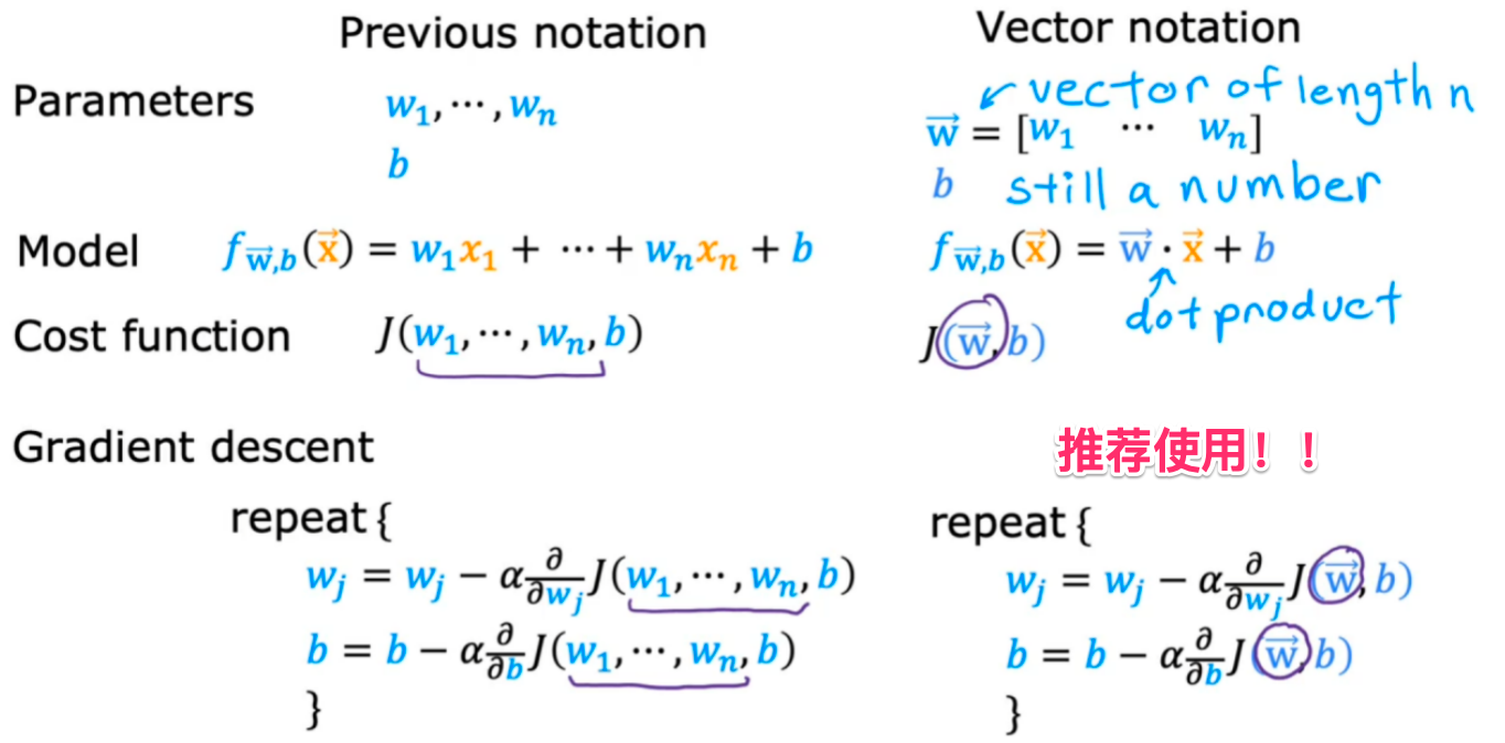
2.单特征梯度下降和多特征梯度下降对比

3.多特征线性回归模型实验(C1_W2_Lab02_Multiple_Variable_Soln)
(1).背景及提供的数据集
你将使用房价预测的例子。训练数据集包含三个示例(三行数据),具有四个特征(大小、卧室、楼层和年龄),如下表所示。请注意,与之前的实验不同,这里的尺寸是平方英尺,而不是1000平方英尺。这导致了一个问题,你将在下一个实验中解决!


# 向量化
X_train = np.array([[2104, 5, 1, 45], [1416, 3, 2, 40], [852, 2, 1, 35]])
y_train = np.array([460, 232, 178])
(2).参数初始化
b_init = 785.1811367994083
w_init = np.array([ 0.39133535, 18.75376741, -53.36032453, -26.42131618])
print(f"w_init shape: {w_init.shape}, b_init type: {type(b_init)}")
初始化一个四维向量,对应于数据集的四个维度
(3).实现多维度线性回归模型代价计算

# 实现 (3) 公式的计算
def compute_cost(X, y, w, b):
    """
    compute cost
    Args:
      X (ndarray (m,n)): Data, m examples with n features
      y (ndarray (m,)) : target values
      w (ndarray (n,)) : model parameters
      b (scalar)       : model parameter

    Returns:
      cost (scalar): cost
    """
    m = X.shape[0]
    cost = 0.0
    for i in range(m):
        f_wb_i = np.dot(X[i], w) + b           #(n,)(n,) = scalar (see np.dot)
        cost = cost + (f_wb_i - y[i])**2       #scalar
    cost = cost / (2 * m)                      #scalar
    return cost
测试用初始值w_init和b_init计算代价值
# Compute and display cost using our pre-chosen optimal parameters.
cost = compute_cost(X_train, y_train, w_init, b_init)
print(f'Cost at optimal w : {cost}')
(4).实现多变量线性回归模型梯度计算

# 实现 (6) (7) 公式的计算
def compute_gradient(X, y, w, b):
    """
    Computes the gradient for linear regression
    Args:
      X (ndarray (m,n)): Data, m examples with n features
      y (ndarray (m,)) : target values
      w (ndarray (n,)) : model parameters
      b (scalar)       : model parameter

    Returns:
      dj_dw (ndarray (n,)): The gradient of the cost w.r.t. the parameters w.
      dj_db (scalar):       The gradient of the cost w.r.t. the parameter b.
    """
    m,n = X.shape           #(number of examples, number of features)
    dj_dw = np.zeros((n,))
    dj_db = 0.


    for i in range(m):
        err = (np.dot(X[i], w) + b) - y[i]
        for j in range(n):
            dj_dw[j] = dj_dw[j] + err * X[i, j]
        dj_db = dj_db + err
    dj_dw = dj_dw / m
    dj_db = dj_db / m

    return dj_db, dj_dw
测试一下初始情况下的梯度
#Compute and display gradient
tmp_dj_db, tmp_dj_dw = compute_gradient(X_train, y_train, w_init, b_init)
print(f'dj_db at initial w,b: {tmp_dj_db}')
print(f'dj_dw at initial w,b: \n {tmp_dj_dw}')
(5).将上面步骤(3)(4)实现的代码代入梯度下降算法的上面公式(5)中
def gradient_descent(X, y, w_in, b_in, cost_function, gradient_function, alpha, num_iters):
    """
    Performs batch gradient descent to learn theta. Updates theta by taking
    num_iters gradient steps with learning rate alpha

    Args:
      X (ndarray (m,n))   : Data, m examples with n features
      y (ndarray (m,))    : target values
      w_in (ndarray (n,)) : initial model parameters
      b_in (scalar)       : initial model parameter
      cost_function       : function to compute cost
      gradient_function   : function to compute the gradient
      alpha (float)       : Learning rate
      num_iters (int)     : number of iterations to run gradient descent

    Returns:
      w (ndarray (n,)) : Updated values of parameters
      b (scalar)       : Updated value of parameter
      """

    # An array to store cost J and w's at each iteration primarily for graphing later
    J_history = []
    w = copy.deepcopy(w_in)  #avoid modifying global w within function
    b = b_in

    for i in range(num_iters):


        # Calculate the gradient and update the parameters
        dj_db,dj_dw = gradient_function(X, y, w, b)   ##None


        # Update Parameters using w, b, alpha and gradient
        w = w - alpha * dj_dw               ##None
        b = b - alpha * dj_db               ##None

        # Save cost J at each iteration
        if i<100000:      # prevent resource exhaustion
            J_history.append( cost_function(X, y, w, b))


        # Print cost every at intervals 10 times or as many iterations if < 10
        if i% math.ceil(num_iters / 10) == 0:
            print(f"Iteration {i:4d}: Cost {J_history[-1]:8.2f}   ")

    return w, b, J_history #return final w,b and J history for graphing
(6).梯度下降算法测试执行并预测
# initialize parameters
initial_w = np.zeros_like(w_init)
initial_b = 0.
# some gradient descent settings
iterations = 1000
alpha = 5.0e-7
# run gradient descent
w_final, b_final, J_hist = gradient_descent(X_train, y_train, initial_w, initial_b,
                                                    compute_cost, compute_gradient,
                                                    alpha, iterations)
print(f"b,w found by gradient descent: {b_final:0.2f},{w_final} ")
m,_ = X_train.shape
for i in range(m):
    print(f"prediction: {np.dot(X_train[i], w_final) + b_final:0.2f}, target value: {y_train[i]}")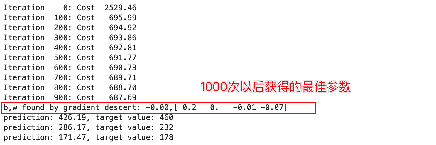
(7).回顾结果
# plot cost versus iteration
fig, (ax1, ax2) = plt.subplots(1, 2, constrained_layout=True, figsize=(12, 4))
ax1.plot(J_hist)
ax2.plot(100 + np.arange(len(J_hist[100:])), J_hist[100:])
ax1.set_title("Cost vs. iteration");  ax2.set_title("Cost vs. iteration (tail)")
ax1.set_ylabel('Cost')             ;  ax2.set_ylabel('Cost')
ax1.set_xlabel('iteration step')   ;  ax2.set_xlabel('iteration step')
plt.show()
后面将会对这个问题进行优化。
六、总结
在这一章中学习了多特征的线性回归模型的应用场景、多特征的线性回归模型梯度下降法、多特征变量的向量表示并强调了向量化操作在效率提升上的重要性。
接着,文章详细比较了单特征和多特征梯度下降的区别,以及传统设置变量法与向量表示的异同。
最后,通过实际实验,展示了如何运用numpy包对向量或矩阵的各种处理操作,如何运用多特征的线性回归模型梯度下降法迭代计算令代价最小的多个特征参数的值。
整篇文章系统地概述了梯度下降在多元线性回归中的应用。
下一章将学习 特征缩放。


 1155
1155


 被折叠的 条评论
为什么被折叠?
被折叠的 条评论
为什么被折叠?
 到【灌水乐园】发言


