python中numpy包

最新推荐文章于 2024-05-16 21:41:01 发布

herry57

最新推荐文章于 2024-05-16 21:41:01 发布

阅读量471

点赞数 2

分类专栏：数学建模文章标签： python 开发语言

本文链接：https://blog.csdn.net/herry57/article/details/125216962

版权

数学建模专栏收录该内容

23 篇文章 8 订阅

订阅专栏

0.概念

Numpy支持常见的数组和矩阵操作。对于同样的数值计算任务，使用Numpy比直接使用Python要简洁的多。

1.属性

import numpy as np
score=np.array([[80, 89, 86, 67, 79],
[78, 97, 89, 67, 81],
[90, 94, 78, 67, 74],
[91, 91, 90, 67, 69],
[76, 87, 75, 67, 86],
[70, 79, 84, 67, 84],
[94, 92, 93, 67, 64],
[86, 85, 83, 67, 80]])
print(score.shape)  #矩阵形状的大小：(8, 5)
print(score.ndim)   #数组维数:2维
print(score.size)   #数组中的元素数量:40
print(score.itemsize)  #一个数组元素的长度（字节）:4
print(score.dtype)     #数组元素的类型:int32

2.操作

2.1生成0，1矩阵

import numpy as np
a=np.ones([4,3])
b=np.zeros([4,2])
c=np.zeros_like(a)

2.2生成固定范围的数组

2.2.1等差数列

import numpy as np
a=np.linspace(0,100,11) #指定数量
print(a) #[  0.  10.  20.  30.  40.  50.  60.  70.  80.  90. 100.]
b=np.arange(10, 50, 2) #指定步长
print(b) # [10 12 14 16 18 20 22 24 26 28 30 32 34 36 38 40 42 44 46 48]

2.2.2等比数列

import numpy as np
c=np.logspace(0, 2, 3)
print(c) #[  1.  10. 100.]

2.3随机数组

2.3.1正态分布

import numpy as np
import matplotlib.pyplot as plt
x1 = np.random.normal(1.75, 1, 100000000) # 生成均值为1.75，标准差为1的正态分布数据，100000000个
# 1）创建画布
plt.figure(figsize=(20, 10), dpi=100)
# 2）绘制直方图
plt.hist(x1, 1000) #这个参数指定bin(箱子)的个数,也就是总共有几条条状图
# 3）显示图像
plt.show()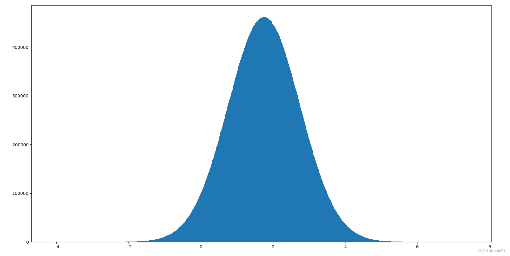

2.3.2均匀分布

import matplotlib.pyplot as plt
import numpy as np
# 生成均匀分布的随机数
x2 = np.random.uniform(-1, 1, 100000000) #-1下界，1上界
# 画图看分布状况
# 1）创建画布
plt.figure(figsize=(10, 10), dpi=100)
# 2）绘制直方图
plt.hist(x=x2, bins=1000) # x代表要使用的数据，bins表示要划分区间数
# 3）显示图像
plt.show()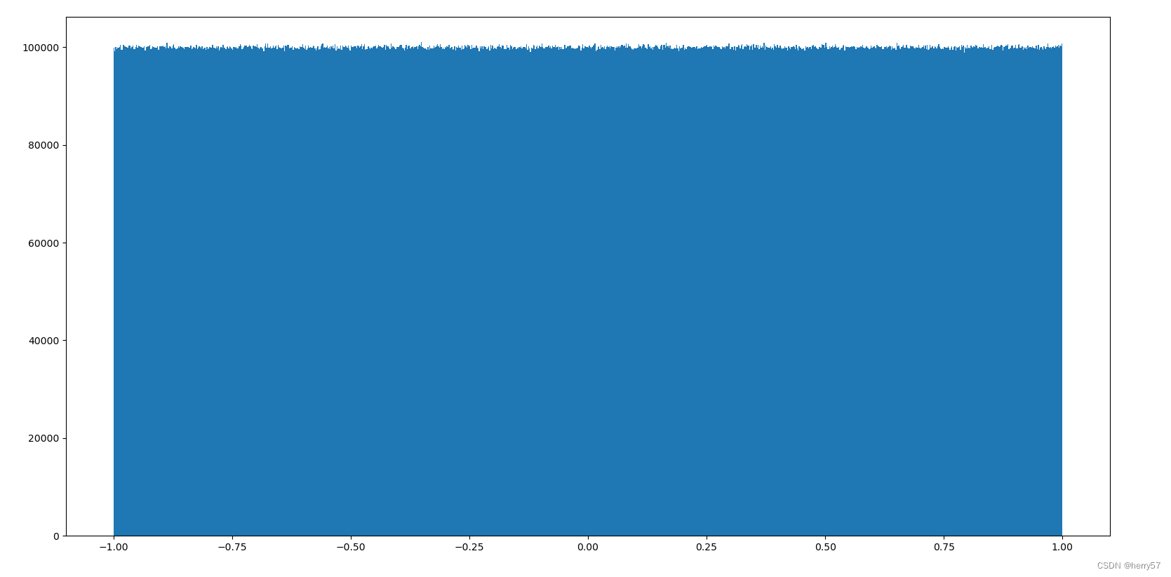

3.索引与切片

import numpy as np
score=np.array([[80, 89, 86, 67, 79],
[78, 97, 89, 67, 81],
[90, 94, 78, 67, 74],
[91, 91, 90, 67, 69],
[76, 87, 75, 67, 86],
[70, 79, 84, 67, 84],
[94, 92, 93, 67, 64],
[86, 85, 83, 67, 80]])
print(score[0,1:3]) #[89 86]

import numpy as np
a1 = np.array([ [[1,2,3],[4,5,6]], [[12,3,34],[5,6,7]]])
print(a1[0,0,2]) #3

4.运算

4.1逻辑运算

import numpy as np
score = np.random.randint(40, 100, (10, 5))
print(score)
test_score = score[6:10, 0:5] #取最后四行
print(test_score>60) #逻辑判断, 如果大于60就标记为True 否则为False
test_score[test_score > 60] = 1
print(test_score)

4.2通用判断函数

print(np.all(score[0:2, :] > 60) )#判断前两行全部> 60
print(np.any(score[0:2, :] > 80)) #判断前两行> 80

4.3np.where（三元运算符）

print(np.where(score[:4,:4]>60,1,0)) #判断四行中，大于60的置为1，否则为0
print(np.where(np.logical_and(score[:4,:4] > 60,score[:4,:4]< 90), 1, 0)) #中大于60且小于90的换为1，否则为0
print(np.where(np.logical_or(score[:4,:4] > 90, score[:4,:4] < 60), 1, 0)) #大于90或小于60的换为1，否则为0

5.统计计算

temp = score[:4, 0:5]
print("前四名学生,各科成绩的最大分：{}".format(np.max(temp, axis=0))) #默认行，axis=1默认列
print("前四名学生,各科成绩的最小分：{}".format(np.min(temp, axis=0)))
print("前四名学生,各科成绩波动情况：{}".format(np.std(temp, axis=0)))
print("前四名学生,各科成绩的平均分：{}".format(np.mean(temp, axis=0)))
print("前四名学生，各科成绩最高分对应的学生下标：{}".format(np.argmax(temp, axis=0)))

结果：

前四名学生,各科成绩的最大分：[63 90 98 99 93]
前四名学生,各科成绩的最小分：[50 57 64 40 74]
前四名学生,各科成绩波动情况：[ 4.656984   15.10794493 12.91317157 21.61452058  7.49583218]
前四名学生,各科成绩的平均分：[56.75 72.5  76.5  73.25 81.75]
前四名学生，各科成绩最高分对应的学生下标：[1 3 1 0 0]

6.数组间的运算

import numpy as np
arr = np.array([[1, 2, 3, 2, 1, 4], [5, 6, 1, 2, 3, 1]])
print(arr + 1)
print(arr / 2)
a = np.array([[80, 86],
[82, 80],
[85, 78],
[90, 90],
[86, 82],
[82, 90],
[78, 80],
[92, 94]])
b = np.array([[0.7], [0.3]])
print(np.dot(a,b))

结果：

[[2 3 4 3 2 5]
 [6 7 2 3 4 2]]
[[0.5 1.  1.5 1.  0.5 2. ]
 [2.5 3.  0.5 1.  1.5 0.5]]
[[81.8]
 [81.4]
 [82.9]
 [90. ]
 [84.8]
 [84.4]
 [78.6]
 [92.6]]