Julia数据可视化：GR.jl包的使用

一、介绍

GR本质上是基于图形内核系统(GKS)和OpenGL的实现。GR.jl是对GR的包装，相比其他Julia绘图库，它的优点是快速。

GR官网：Julia Package GR — GR Framework 0.71.7 documentation

GR.jl GitHub地址：GitHub - jheinen/GR.jl: Plotting for Julia based on GR

二、基本绘图

可用接口如下：

colormap,
figure,
gcf,
hold,
usecolorscheme,
subplot,
plot,
oplot,
stairs,
scatter,
stem,
barplot,
histogram,
polarhistogram,
contour,
contourf,
hexbin,
heatmap,
polarheatmap,
wireframe,
surface,
volume,
plot3,
scatter3,
title,
redraw,
xlabel,
ylabel,
drawgrid,
xticks,
yticks,
zticks,
xticklabels,
yticklabels,
legend,
xlim,
ylim,
savefig,
meshgrid,
meshgrid,
peaks,
imshow,
isosurface,
cart2sph,
sph2cart,
polar,
trisurf,
tricont,
shade,
setpanzoom,
mainloop

1. 折线图

using GR
plot(rand(30))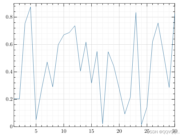

多条折线 

using GR

# 创建数据
x = collect(range(-2, 2, length=40))
y = 2 .* x .+ 4

# 第一条折线
plot(x, y)

# 第二条折线
oplot(x, x -> x^3 + x^2 + x)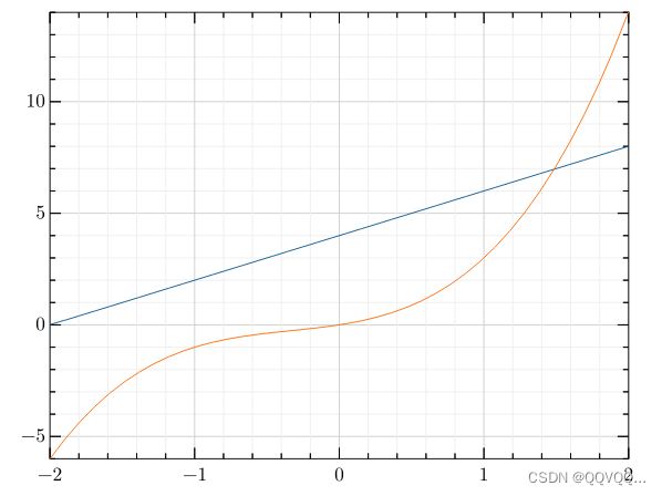

三维曲线

using GR
x = LinRange(0, 30, 1000)
y = cos.(x) .* x
z = sin.(x) .* x
plot3(x, y, z)

2. 条形图

垂直条形图

using GR
population = Dict(
    "Africa" => 216,
    "America" => 316,
    "Asia" => 436,
    "Europe" => 39,
    "Oceania" => 38
)
barplot(keys(population), values(population))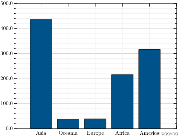

 

 水平条形图 

using GR
population = Dict(
    "Africa" => 216,
    "America" => 316,
    "Asia" => 436,
    "Europe" => 39,
    "Oceania" => 38
)
barplot(keys(population), values(population), horizontal=true)

3. 直方图

using GR
histogram(randn(10000))

 

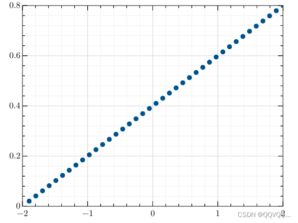
4. 散点图

using GR

# 创建数据
x = LinRange(-2, 2, 40)
y = 0.2 .* x .+ 0.4

# 方式一
scatter(x, y)

# 方式二
scatter(x, x -> 0.2 * x + 0.4)

using GR

 x = 2 .* rand(100) .- 1
 y = 2 .* rand(100) .- 1
 z = 2 .* rand(100) .- 1
 c = 999 .* rand(100) .+ 1

 scatter3(x, y, z, c)

5. 茎段图

using GR

x = LinRange(-2, 2, 40)
y = 0.2 .* x .+ 0.4

stem(x, y)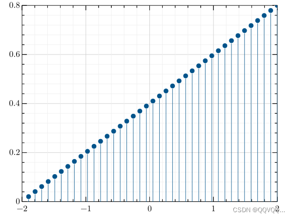

 6. 其他图形

using GR

subplot(2, 3, 1)
hexbin(randn(100), randn(100))

subplot(2, 3, 2)
x = LinRange(-2, 2, 40)
y = LinRange(0, pi, 20)
z = sin.(x') .+ cos.(y)
contour(x, y, z)

subplot(2, 3, 3)
x = LinRange(-2, 2, 40)
y = LinRange(0, pi, 20)
z = sin.(x') .+ cos.(y)
contourf(x, y, z)

subplot(2, 3, 4)
x = 8 .* rand(100) .- 4
y = 8 .* rand(100) .- 4
z = sin.(x) + cos.(y)
tricont(x, y, z)

subplot(2, 3, 5)
x = LinRange(-2, 2, 40)
y = LinRange(0, pi, 20)
z = sin.(x') .+ cos.(y)
surface(x, y, z)

subplot(2, 3, 6)
x = 8 .* rand(100) .- 4
y = 8 .* rand(100) .- 4
z = sin.(x) .+ cos.(y)
trisurf(x, y, z)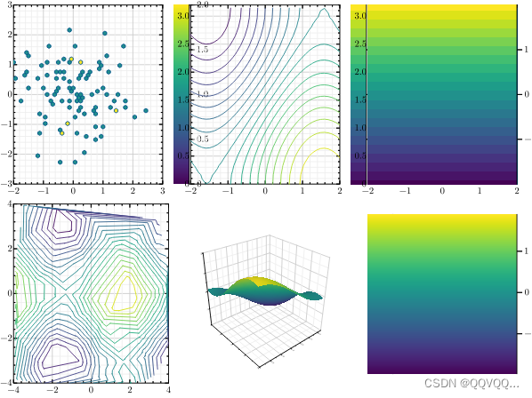

 三、属性设置

1. 图片大小

figsize 关键字可用于设置图片大小，示例如下:

# 方法一
figure(figsize=(5,3))

# 方法二
plot([1, 2, 3],figsize=(5,3))

2. 标题

figure(title="Example Figure") # 设置图像标题
title("Example Plot") # 设置图像标题，同上

3. 坐标轴

xlabel("x")  # 设置x轴标签
ylabel("y")  # 设置y轴标签
xlim((-1,10))  # 设置x轴的范围
ylim((-1,10))  # 设置y轴的范围

4. 刻度

xticks(0.2)  # 每0.2个单位一个刻度
xticks(0.2, 5)  # 每五个小刻度绘制一个大刻度
yticks(0.2)
yticks(0.2, 5)
zticks(0.2)
zticks(0.2, 5)

5. 网格

grid(false)  # 隐藏网格
grid(true)  # 恢复网格

6. 图例

legend("a", "b")  # 设置图例

7. 颜色

using GR
plot(rand(50), "r")  # 红色
plot(rand(50), "b")  # 蓝色
plot(rand(50), "w")  # 白色
plot(rand(50), "y")  # 黄色
plot(rand(50), "g")  # 绿色

四、其他功能

1. hold()

保存当前绘图

2. redraw()

重置绘图

3. savefig()

保存图片

4. figure()

新建绘图