用TensorFlow构建基础的神经网络(一)：MLP

源代码下载：http://pan.baidu.com/s/1kUAsk5L
作者：XJTU_Ironboy
时间：2017年8月

开头语

  由于最近在学习Deep Learning方面的知识，并尝试着用Google近些年刚提出的TensorFlow框架来搭建各种经典的神经网络，如MLP、LeNet-5、AlexNet、VGG、GoogleNet、ResNet、DenseNet、SqueezeNet，所以在接下来的学习过程中我将逐个地介绍MLP、LeNet-5和AlexNet三个基础的神经网络的结构细节，因为其他的神经网络都可以说是在AlexNet上进行结构的修改而得到的，所以说如果学会了这三个基本网络的构建，那么其他结构的构建就是套路了。

一、MLP

1.单层感知机

  在我的理解中，Deep Learning的学习大多数都是从感知机(perceptron)开始的，因为它是神经网络的开山鼻祖，一种最最简单的神经网络结构。
  感知机是一种二分类模型，输入实例的特征向量，输出实例的±类别。由于这个模型过于简单，懒得废话，还是直接上图吧。

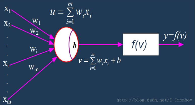
其中输入(Input)是一个m维的向量: $[X_1,X_2,X_3,...,X_i,...,X_m]$，权重(Weight)也是一个m维的向量: $[W_1,W_2,W_3,...,W_i,...,W_m]$，偏置项(Bias)是:$[b]$，输出(Output)是一个标量输出:$y$，激活函数(Activation Function)是: 符号函数（signum：x大于0的时候为1；x等于0的时候为0，x小于0的时候为-1）。

2.多层感知机

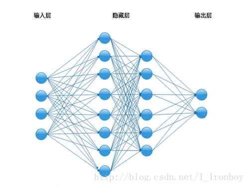
  多层感知器（MLP，Multilayer Perceptron）是一种前馈人工神经网络模型，其将输入的多个数据集映射到单一的输出的数据集上。

  接下来讲一下如何用TensorFlow来实现这个简单的多层感知机(MLP):
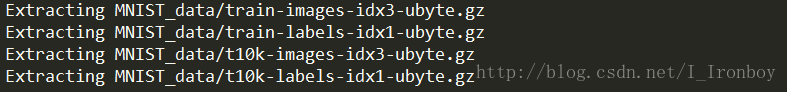
  1.数据库： MNIST数字手写体数据库
  2.编程配置： Python3.5 + TensorFlow1.2.0
  3.结构： 输入层+一个隐含层+输出层
     输入图像大小： $28 \times 28$；
     隐含层神经元个数： 300；
    输出神经元个数： 10；
     激活函数： ReLU
    优化器： Adagrad
    训练集上的batch size： 1000
    测试集上的batch size： 10000
  4.TensorFlow上实现
① 首先，导入tensorflow和MNIST数据集

import tensorflow as tf
# 导入MNIST数字手写体数据库
from tensorflow.examples.tutorials.mnist import input_data
mnist = input_data.read_data_sets("MNIST_data/",one_hot = True)

② 开始定义MLP的整体结构

# 定义输入层、隐含层、输出层的神经元个数
in_units = 784
h1_units = 300
out_units = 10

③ 输入层，with tf.name_scope是TensorFlow中的命名空间，便于在tensorboard可视化整体的结构

# 定义输入层，keep_prob是dropout的比例
with tf.name_scope("input"):
    x = tf.placeholder(tf.float32,[None,in_units])
    y_= tf.placeholder(tf.float32,[None,out_units])
keep_prob = tf.placeholder(tf.float32)

④ 隐含层：权重、偏置的初始值都是正态分布的随机数

# 定义隐含层的权重、偏置、激活函数
with tf.name_scope("hidden_layer1"):
    with tf.name_scope("w1"): 
        w1 = tf.Variable(tf.random_normal([in_units,h1_units],stddev = 0.1))
        tf.summary.histogram('Weight1',w1)
    with tf.name_scope("b1"): 
        b1 = tf.Variable(tf.zeros([h1_units])) + 0.01
        tf.summary.histogram('biases1',b1)
    with tf.name_scope("w1_b1"):
        hidden1 = tf.nn.relu(tf.matmul(x,w1) + b1)
        tf.summary.histogram('output1',hidden1)

⑤ 输出层：权重、偏置的初始值都是正态分布的随机数

# 定义输出层的权重、偏置、激活函数
with tf.name_scope("output_layer"):
    with tf.name_scope("w2"): 
        w2 = tf.Variable(tf.random_normal([h1_units,out_units],stddev = 0.1))
        tf.summary.histogram('Weight2',w2)
    with tf.name_scope("b2"): 
        b2 = tf.Variable(tf.zeros([out_units]))
        tf.summary.histogram('biases2',b2)
    with tf.name_scope("w2_b2"):
        hidden1_drop = tf.nn.dropout(hidden1,keep_prob)
with tf.name_scope("output"):
    y = tf.nn.softmax(tf.matmul(hidden1_drop,w2)+b2)
    tf.summary.histogram('output',y)

⑥ 损失函数、准确率、优化器

# 定义损失函数———交叉熵
with tf.name_scope("loss"):
    cross_entropy = tf.reduce_mean(-tf.reduce_sum(y_*tf.log(y),reduction_indices = [1]))
    tf.summary.scalar('cross_entropy', cross_entropy)
# 计算准确率
with tf.name_scope("accuracy"):
    correct_prediction = tf.equal(tf.argmax(y,1),tf.argmax(y_,1))
    accuracy = tf.reduce_mean(tf.cast(correct_prediction,tf.float32))
# 定义优化器——Adagrad，和学习率:0.3
with tf.name_scope("train"):    
    train_step = tf.train.AdagradOptimizer(0.3).minimize(cross_entropy)

⑦ 框架搭好了，正式开始计算

# 初始化所有的变量
init = tf.global_variables_initializer() 
# 开始导入数据，正式计算，迭代3000步，训练时batch size=100
with tf.Session() as sess:
    sess.run(init)
    merge = tf.summary.merge_all()
    writer = tf.summary.FileWriter("log",sess.graph)
    for i in range(3000):
        batch_xs,batch_ys = mnist.train.next_batch(1000)
        sess.run(train_step,feed_dict = {x:batch_xs,y_:batch_ys,keep_prob:0.75})
        loss_run = sess.run(cross_entropy,feed_dict = {x:batch_xs,y_:batch_ys,keep_prob:0.75})
        accuracy_run = sess.run(accuracy,feed_dict = {x:batch_xs,y_:batch_ys,keep_prob:0.75})
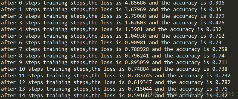
        print('after %d steps training steps,the loss is %g and the accuracy is %g'%(i,loss_run,accuracy_run))
        result = sess.run(merge,feed_dict = {x:batch_xs,y_:batch_ys,keep_prob:1})
        writer.add_summary(result,i)
        # 训练完后直接加载测试集数据，进行测试
        if i == 2999:
            loss_run = sess.run(cross_entropy,feed_dict = {x:mnist.test.images,y_:mnist.test.labels,keep_prob:1})
            accuracy_run = sess.run(accuracy,feed_dict = {x:mnist.test.images,y_:mnist.test.labels,keep_prob:1})
            print('the loss in test dataset is %g and the accuracy in test dataset is %g'%(loss_run,accuracy_run))

  5 .运行结果：

…

…

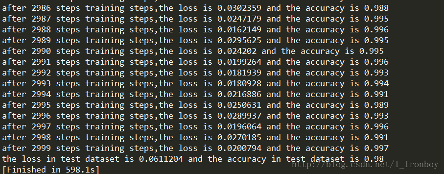
   测试集上的准确度：98.00%
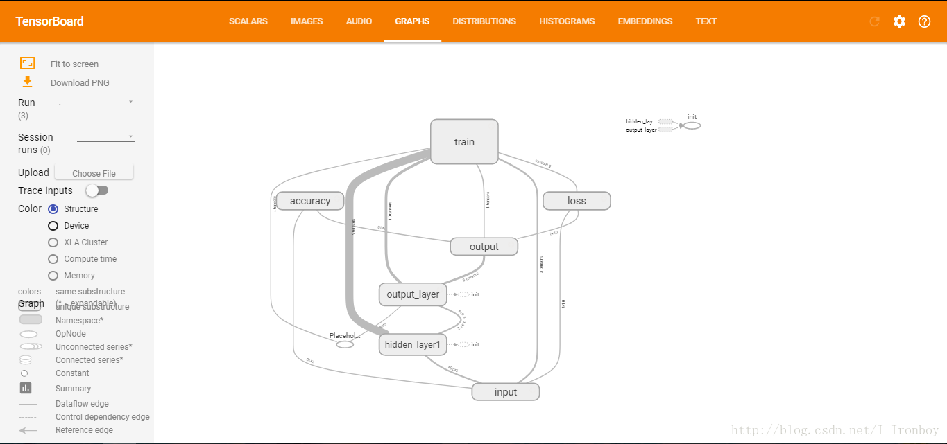
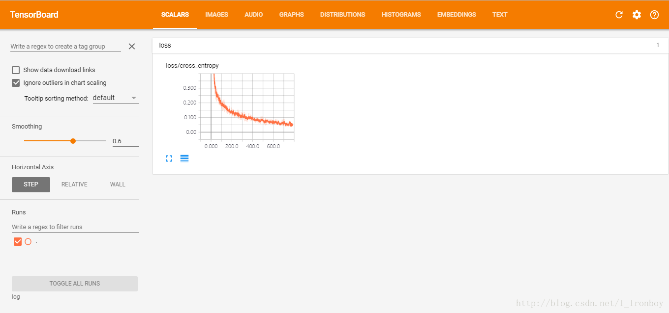
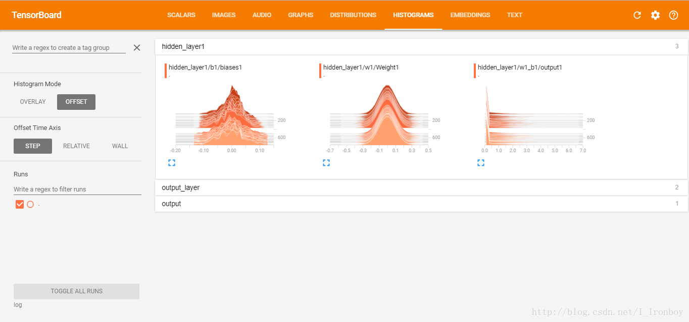
  6. TensorBoard可视化：
① 在MLP.py程序的所在文件夹下打开cmd窗口(针对Windows)
方法一：打开cmd，然后用“cd + 路径”的方式找到该位置
方法二：定位到MLP.py所在文件的位置，点击左上角的“文件”，然后点击“打开命令提示符”
② 输入： tensorboard - -logdir=log ，回车

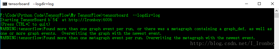
③ 复制上面的地址到浏览器，如我这上面的地址是:http://Ironboy:6006
④ 可视化结果：