Machine Learning in Action 读书笔记---第3章决策树

最新推荐文章于 2022-04-14 13:12:36 发布

dongyuyuu

最新推荐文章于 2022-04-14 13:12:36 发布

阅读量194

点赞数

分类专栏：【机器学习】文章标签：决策树机器学习

本文链接：https://blog.csdn.net/id__39/article/details/118462696

版权

【机器学习】专栏收录该内容

14 篇文章 0 订阅

订阅专栏

Machine Learning in Action 读书笔记

第3章决策树

文章目录

Machine Learning in Action 读书笔记
一、决策树算法简介
- 1 决策树的构造
- 2 决策树的一般流程
二、决策树的构造过程
三、实例：使用决策树预测隐形眼镜类型
四、本章小结
五、全部代码

一、决策树算法简介

经常使用决策树来处理分类问题，决策树也是最经常使用的数据挖掘算法。决策树相比于第二章中的k近邻算法：k近邻不能给出数据的内在含义，决策树的主要优势就在于数据形式非常容易理解。

决策树算法能够读取数据集合，决策树的一个重要任务是为了理解数据中所蕴含的知识信息，因此决策树可以使用不熟悉的数据集合，并从中提取出一系列规则，这些机器根据数据集创建规则的过程，就是机器学习的过程。

1 决策树的构造

优点：计算复杂度不高，输出结果易于理解，对中间值的缺失不敏感，可以处理不相关特征的数据。
缺点：可能会产生过度匹配问题
适用数据类型：数值型和标称型

2 决策树的一般流程

收集数据：可以使用任何方法
准备数据：树构造算法只适用于标称型数据，因此数值型数据必须离散化
分析数据：可以使用任何方法，构造树完成后，我们应该检查图型是否符合预期
训练算法：构造树的数据结构
测试算法：使用经验树计算错误率
使用算法：此步骤可以适用于任何监督学习算法，而使用决策树可以更好地理解数据的内在含义

思考一个问题：如何从一堆原始数据中构造决策树？

在函数中调用的数据需要满足的条件：

数据必须是一种由列表元素组成的列表，而且所有列表元素都要具有相同的数据长度
数据的最后一列或者每个实例的最后一个元素是当时实例的列表标签（决策树中的叶子节点）

二、决策树的构造过程

1. 划分数据集

在构造决策树时，我们需要解决的第一个问题就是，当前数据集上哪个特征在划分数据分类时起决定性作用？为了找到决定性的特征，划分出最好的结果，我们必须评估每一个特征。

划分数据集的最大原则是：将无序数据变得更加有序。本章使用ID3（Iterative Dichotomiser 3，迭代二分器）算法划分数据集。根据未使用过的特征计算熵H(S)（也称为香农熵）和信息增益IG(S)，小熵或者拥有最大信息增益的特征为划分数据集的最好选择。

计算给定数据集的香农熵代码如下：

'''创建数据集'''
def createDataSet():
    dataSet = [[1, 1, 'yes'],
               [1, 1, 'yes'],
               [1, 0, 'no'],
               [0, 1, 'no'],
               [0, 1, 'no']
               ]
    labels = ['no surfacing', 'flippers']  # 两个判断特征：不浮出水面是否可以生存，是否有脚蹼，最后一列为属性，yes表示是鱼类，no表示非鱼类
    return dataSet, labels

'''计算给定数据集的香农熵'''
def calShannonEnt(dataSet):
    numEntries = len(dataSet)
    # print(numEntries)
    labelCounts = {}
    for featVec in dataSet:
        currentLabel = featVec[-1]
        if currentLabel not in labelCounts.keys():
            labelCounts[currentLabel]  = 0
        labelCounts[currentLabel] += 1
    shannonEnt = 0.0
    for key in labelCounts:
        prob = float(labelCounts[key])/numEntries
        shannonEnt -= prob * log(prob, 2)
    return shannonEnt

按照给定特征划分数据集：

''' 按照给定特征划分数据集 '''
def splitDataSet(dataSet, axis, value): # 三个参数：待划分数据集，划分数据集的特征，需要返回的特征值
    retDataSet = []
    for featVec in dataSet:
        if featVec[axis] == value:
            reducedFeatVec = featVec[:axis]
            # print(featVec[:axis])
            reducedFeatVec.extend(featVec[axis+1:])
            retDataSet.append(reducedFeatVec)
    return retDataSet

选择最好的数据集划分方式：

''' 选择最好的数据集划分方式 '''
def chooseBestFeatureToSplit(dataSet):
    numFeatures = len(dataSet[0]) - 1
    baseEntropy = calShannonEnt(dataSet) # 计算整个数据集的香农熵
    bestInfoGain = 0.0 ; bestFeature = -1
    for i in range(numFeatures):  # 遍历数据集中的所有特征
        featList = [example[i] for example in dataSet]
        uniqueVals = set(featList)    # 利用集合消除相同的特征值
        newEntropy = 0.0
        for value in uniqueVals:
            subDataSet = splitDataSet(dataSet, i, value)
            prob = len(subDataSet)/float(len(dataSet))
            newEntropy += prob * calShannonEnt(subDataSet)  # 计算新数据集的香农熵（对所有特征的熵值求和）
        infoGain = baseEntropy - newEntropy  # 与划分之后的数据集的熵值进行比较，获得最大信息增益
        if (infoGain > bestInfoGain):
            bestInfoGain = infoGain
            bestFeature = i
    return bestFeature # 返回最好特征的索引值

2.递归构建决策树

使用递归创建树，递归结束的两个条件：

程序遍历完所有划分数据集的属性
或者每个分支下的所有实例都具有相同的分类（叶子节点的类型已经确定）

创建树的函数代码：

'''学习了如何度量数据集的信息熵 和 如何有效的划分数据集后，递归构建决策树（以字典形式存储）'''
def createTree(dataSet, labels):  # 数据集和标签列表
    classList = [example[-1] for example in dataSet]   # 数据集的所有类标签
    # print("classList:", classList)
    if classList.count(classList[0]) == len(classList):  # 递归函数的第一个停止条件：所有类标签完全相同，则直接返回该类标签
        # print(classList.count(classList[0]), len(classList))
        return classList[0]
    if len(dataSet[0]) == 1:  # 递归函数的第二个停止条件：使用完了所有特征，只剩下最后一列的眼镜类型
        return majorityCnt(classList)  # 选择多的
    bestFeat = chooseBestFeatureToSplit(dataSet)
    bestFeatLabel = labels[bestFeat]
    myTree = {bestFeatLabel:{}}   # 使用字典类型存储树的信息, 获得的最好特征作为树的根
    del(labels[bestFeat])
    featValues = [example[bestFeat] for example in dataSet]  # featValues存储树边上的值
    uniqueVals = set(featValues) # 通过集合消除重复的特征值
    for value in uniqueVals: # 以根节点为例子，这里的value为reduced和normal
        subLabels = labels[:]
        myTree[bestFeatLabel][value] = createTree(splitDataSet(dataSet, bestFeat, value), subLabels)
    return myTree

如果数据集已经处理了所有属性，但是类标签依然不是唯一的，此时我们需要决定如何定义该叶子节点，在这种情况下，通常会采用多数表决的方法决定叶子节点的分类。代码如下：

'''如果数据集已经处理了所有属性，但是类标签依然不是唯一的，此时采用多数表决的方法决定该叶子节点的分类'''
def majorityCnt(classList):
    classCount = {}
    for vote in classList:
        if vote not in classCount.keys():
            classCount[vote] = 0
        classCount[vote] += 1
    sortedClassCount = sorted(classCount.items(), key=operator.itemgetter(1), reverse=True)
    return sortedClassCount[0][0]

3.在python中使用matplotlib注解绘制树形图

决策树的主要优点就是直观易于理解，如果不能将其直观地显示出来，就无法发挥其优势。
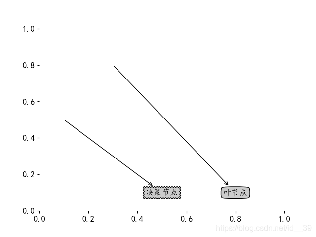
使用文本注解绘制树节点：

import matplotlib.pyplot as plt

plt.rcParams['font.sans-serif'] = ['KaiTi', 'SimHei', 'FangSong']  # 汉字字体,优先使用楷体，如果找不到楷体，则使用黑体
plt.rcParams['font.size'] = 12  # 字体大小
plt.rcParams['axes.unicode_minus'] = False  # 正常显示负号


decisionNode = dict(boxstyle="sawtooth", fc="0.8") # 判断节点设置为光滑框
leafNode = dict(boxstyle="round4", fc="0.8")    # 叶子节点设置为波浪线框
arrow_args = dict(arrowstyle="<-")  #定义箭头类型

def plotNode(nodeTxt, centerPt, parentPt, nodeType):  #  createPlot.ax1为全局变量，绘制图像的句柄
    createPlot.ax1.annotate(nodeTxt, xy=parentPt, xycoords='axes fraction',\
                            xytext=centerPt, textcoords='axes fraction',\
                            va="center", ha="center", bbox=nodeType, arrowprops=arrow_args)

def createPlot():
    '''下面注释代码用于测试'''
    fig = plt.figure(1, facecolor='white')
    fig.clf()
    createPlot.ax1 = plt.subplot(111, frameon=False)   # frameon表示是否绘制坐标轴矩形
    plotNode('决策节点', (0.5, 0.1), (0.1, 0.5), decisionNode)
    plotNode('叶节点', (0.8, 0.1), (0.3, 0.8), leafNode)
    plt.show()

绘制出的图像如下图所示：
在这里插入图片描述

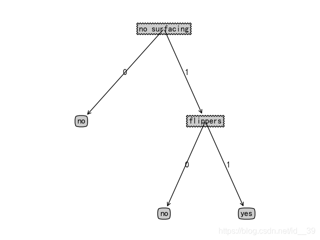
4.判断是否鱼类实例树形图绘制

为了保证绘制树的比例，绘制注解树的第一步是：获取树的叶子节点数和树的层数
叶子节点数用于确定x轴的长度，层数用于确定y轴的高度。

'''获取树的叶子节点数'''
def getNumLeafs(myTree):
    numLeafs = 0
    firstStr = list(myTree.keys())[0]
    # print('firstStr---->', firstStr)
    secondDict = myTree[firstStr]
    # print('secondDict----->', secondDict)
    for key in secondDict.keys():
        if type(secondDict[key]).__name__ == 'dict':   # 测试节点的数据类型是否为字典，继续调用函数
            numLeafs += getNumLeafs(secondDict[key])
        else:
            numLeafs += 1
    return numLeafs
'''获取树的深度'''
def getTreeDepth(myTree):
    maxDepth = 0
    firstStr = list(myTree.keys())[0]
    secondDict = myTree[firstStr]
    for key in secondDict.keys():
        if type(secondDict[key]).__name__ == 'dict':   # 测试节点的数据类型是否为字典，继续调用函数
            thisDepth = 1 + getTreeDepth(secondDict[key])
        else:
            thisDepth = 1
        if thisDepth > maxDepth:
            maxDepth = thisDepth
    return maxDepth

绘制决策树：

def plotMidText(cntrPt, parentPt, txtString):
    xMid = (parentPt[0] - cntrPt[0])/2.0 + cntrPt[0]
    yMid = (parentPt[1] - cntrPt[1]) / 2.0 + cntrPt[1]
    createPlot.ax1.text(xMid, yMid, txtString)

def plotTree(myTree, parentPt, nodeTxt):
    numLeafs = getNumLeafs(myTree)   # 计算树的宽度 3
    depth = getTreeDepth(myTree)     # 计算树的高度 2
    firstStr = list(myTree.keys())[0]
    # plotTree.totalW存储树的宽度，plotTree.totalD存储树的高度， 使用两个变量计算树节点的摆放位置
    # plotTree.xOff 和 plotTree.yOff追踪已经绘制的节点位置，以及放置下一个节点的恰当位置
    cntrPt = (plotTree.xOff + (1.0 + float(numLeafs))/2.0/plotTree.totalW, plotTree.yOff)
    print(cntrPt)
    plotMidText(cntrPt, parentPt, nodeTxt)   # 计算父节点和子节点的中间位置
    plotNode(firstStr, cntrPt, parentPt, decisionNode)
    secondDict = myTree[firstStr]
    plotTree.yOff = plotTree.yOff - 1.0/plotTree.totalD   # 按比例减少plotTree.yOff，并标注此处将要绘制子节点（自顶向下画，所以需要依次递减y坐标值）
    for key in secondDict.keys():
        if type(secondDict[key]).__name__ == 'dict':
            plotTree(secondDict[key], cntrPt, str(key))
        else:
            plotTree.xOff = plotTree.xOff + 1.0/plotTree.totalW
            plotNode(secondDict[key], (plotTree.xOff, plotTree.yOff), cntrPt,leafNode)
            plotMidText((plotTree.xOff, plotTree.yOff), cntrPt, str(key))
    plotTree.yOff = plotTree.yOff + 1.0/plotTree.totalD

def createPlot(inTree):  # 创建绘图区，计算树形图的全局尺寸
    fig = plt.figure(1, facecolor='white')   # 创建画布
    fig.clf() # 清除画布内容
    axprops = dict(xticks=[], yticks=[])  # 定义横纵坐标轴
    # print(axprops) # {'xticks': [], 'yticks': []}
    # createPlot.ax1 = plt.subplot(111, frameon=False, **axprops)  # 绘制图像，无边框，无坐标轴
    createPlot.ax1 = plt.subplot(111, frameon=False)  # 绘制图像，无边框，有坐标轴
    plotTree.totalW = float(getNumLeafs(inTree))  # 全局变量宽度 等于 叶子数
    plotTree.totalD = float(getTreeDepth(inTree))  # 全局变量深度 等于 树的深度
    print(plotTree.totalW, plotTree.totalD)   # 3.0 2.0
    plotTree.xOff = -0.5/plotTree.totalW    # 图像的横纵坐标都在0到1之间，
    plotTree.yOff = 1.0
    # print(plotTree.xOff, plotTree.yOff)  #  -0.16666666666666666 1.0
    plotTree(inTree, (0.5, 1.0), '')
    plt.show()

绘制出的图如下图所示：
在这里插入图片描述
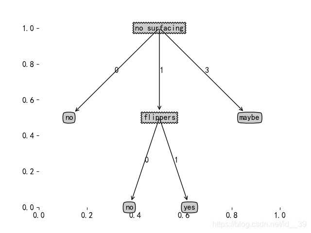
修改字典中一项类型，是鱼类为可能是鱼类，绘制出的决策树如下图：

5.测试算法：使用决策树执行分类

使用决策树的分类函数：

'''使用决策树的分类函数'''
def classify(inputTree, featLabels, testVec):
    firstStr = list(inputTree.keys())[0]
    secondDict = inputTree[firstStr]
    featIndex = featLabels.index(firstStr)  # 使用index方法查找当前列表中第一个匹配firstStr变量的元素
    # print(featIndex)
    for key in secondDict.keys():
        # print('secondDict.keys:', key)
        if testVec[featIndex] == key:
            if type(secondDict[key]).__name__ == 'dict': # 到达叶子节点，就输出该叶子节点类型，否则进入递归
                classLabel = classify(secondDict[key], featLabels, testVec) # 到达判断节点，进入递归调用
            else:
                classLabel = secondDict[key]
    return classLabel

# 测试算法：使用决策树执行分类
    myTree = retrieveTree(0)
    test = classify(myTree, labels, [1, 1])
    # print(test)  # 输出：no，为非鱼类

6.使用算法：决策树的存储

为了节省计算时间，最好能够在每次执行分类时调用已经构造好的决策树，需要使用python模块pickle序列化对象。序列化对象可以在磁盘上保存对象，并在需要的时候读取出来。（任何对象都可以执行序列化操作，字典对象也不例外）

'''在硬盘上存储决策树分类器'''
def storeTree(inputTree, filename):
    import pickle   # 将对象以文件的形式存放在磁盘上
    fw = open(filename, 'wb')
    pickle.dump(inputTree, fw)   # 序列化对象
    fw.close()

def grabTree(filename):
    import pickle
    fr = open(filename, 'rb+')  # 序列化操作时，文件模式为字节处理
    return pickle.load(fr)  # 反序列化对象，将文件中的数据解析为一个python对象

将分类器存储在硬盘上，而不用每次对数据分类时重新学习一遍，这也是决策树的优点之一。k近邻算法就无法持久化分类器。

三、实例：使用决策树预测隐形眼镜类型

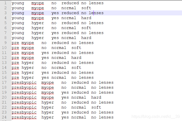
使用数据集如下：一共具有四个特征，最后一列为隐形眼镜类型（hard, soft, no lenses）
在这里插入图片描述

# 隐形眼镜分类案例
    '''
    隐形眼镜的类型包括：硬材质，软材质，不适合佩戴隐形眼镜（hard, soft, no lenses）
    决策树的叶子节点包括这三种类型，要求隐形眼镜的类型属性位于数据集每行的最后一个
    '''
    fr = open('lenses.txt')
    lenses = [inst.strip().split('\t') for inst in fr.readlines()]
    # print(lenses)
    lensesLabels = ['age', 'prescript', 'astigmatic', 'tearRate']  # 用于判断隐形眼镜类型的四个特征：年龄，规定的，散光的，度数
    lensesTree = createTree(lenses, lensesLabels)   # 创建递归树（以字典形式存储）
    # print(lensesTree)   # {'tearRate': {'normal': {'astigmatic': {'yes': {'prescript': ......
    createPlot(lensesTree)  # 根据创建的递归树绘图

画出的决策树如下所示：
在这里插入图片描述
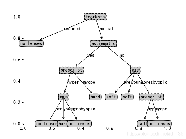
根据上图可知，决策树非常好的匹配了实验数据，但是这些匹配选项太多了，出现了过度匹配问题（overfitting)。为了减少过度匹配问题，我们可以裁剪决策树，去掉一些不必要的叶子节点。如果叶子节点只能增加少许信息，则可以删除该节点，将它并入到其他叶子节点中。

四、本章小结

构建决策树分类器首先需要处理数据集：开始处理数据集时，首先需要测量集合中数据的不一致性，也就是熵；然后寻找最优方案划分数据集，直到数据集中的数据属于同一分类。（第三章中使用ID3算法划分标称型数据集）。第二步：使用递归的方法将数据集转化为决策树，使用字典存储树节点信息。第三步：使用matplotlib注解功能可视化树。最后可能会产生过度匹配问题，可以通过裁剪决策树，合并相邻的无法产生大量信息增益的叶节点，消除过度匹配问题。

五、全部代码

'''trees.py'''
from math import log
import operator
from treePlotter import retrieveTree, createPlot

'''计算给定数据集的香农熵'''
def calShannonEnt(dataSet):
    numEntries = len(dataSet)
    # print(numEntries)
    labelCounts = {}
    for featVec in dataSet:
        currentLabel = featVec[-1]
        if currentLabel not in labelCounts.keys():
            labelCounts[currentLabel]  = 0
        labelCounts[currentLabel] += 1
    shannonEnt = 0.0
    for key in labelCounts:
        prob = float(labelCounts[key])/numEntries
        shannonEnt -= prob * log(prob, 2)
    return shannonEnt

def createDataSet():
    dataSet = [[1, 1, 'yes'],
               [1, 1, 'yes'],
               [1, 0, 'no'],
               [0, 1, 'no'],
               [0, 1, 'no']
               ]
    labels = ['no surfacing', 'flippers']
    return dataSet, labels

''' 按照给定特征划分数据集 '''
def splitDataSet(dataSet, axis, value):
    retDataSet = []
    for featVec in dataSet:
        if featVec[axis] == value:
            reducedFeatVec = featVec[:axis]
            # print(featVec[:axis])
            reducedFeatVec.extend(featVec[axis+1:])
            retDataSet.append(reducedFeatVec)
    return retDataSet

''' 选择最好的数据集划分方式 '''
def chooseBestFeatureToSplit(dataSet):
    numFeatures = len(dataSet[0]) - 1
    baseEntropy = calShannonEnt(dataSet)
    bestInfoGain = 0.0 ; bestFeature = -1
    for i in range(numFeatures):
        featList = [example[i] for example in dataSet]
        uniqueVals = set(featList)
        newEntropy = 0.0
        for value in uniqueVals:
            subDataSet = splitDataSet(dataSet, i, value)
            prob = len(subDataSet)/float(len(dataSet))
            newEntropy += prob * calShannonEnt(subDataSet)
        infoGain = baseEntropy - newEntropy
        if (infoGain > bestInfoGain):
            bestInfoGain = infoGain
            bestFeature = i
    return bestFeature

'''如果数据集已经处理了所有属性，但是类标签依然不是唯一的，此时采用多数表决的方法决定该叶子节点的分类'''
def majorityCnt(classList):
    classCount = {}
    for vote in classList:
        if vote not in classCount.keys():
            classCount[vote] = 0
        classCount[vote] += 1
    sortedClassCount = sorted(classCount.items(), key=operator.itemgetter(1), reverse=True)
    return sortedClassCount[0][0]

'''学习了如何度量数据集的信息熵 和 如何有效的划分数据集后，递归构建决策树（以字典形式存储）'''
def createTree(dataSet, labels):  # 数据集和标签列表
    classList = [example[-1] for example in dataSet]   # 数据集的所有类标签
    # print("classList:", classList)
    if classList.count(classList[0]) == len(classList):  # 递归函数的第一个停止条件：所有类标签完全相同，则直接返回该类标签
        # print(classList.count(classList[0]), len(classList))
        return classList[0]
    if len(dataSet[0]) == 1:  # 递归函数的第二个停止条件：使用完了所有特征，只剩下最后一列的眼镜类型
        return majorityCnt(classList)  # 选择多的
    bestFeat = chooseBestFeatureToSplit(dataSet)
    bestFeatLabel = labels[bestFeat]
    myTree = {bestFeatLabel:{}}   # 使用字典类型存储树的信息, 获得的最好特征作为树的根
    del(labels[bestFeat])
    featValues = [example[bestFeat] for example in dataSet]  # featValues存储树边上的值
    uniqueVals = set(featValues) # 通过集合消除重复的特征值
    for value in uniqueVals: # 以根节点为例子，这里的value为reduced和normal
        subLabels = labels[:]
        myTree[bestFeatLabel][value] = createTree(splitDataSet(dataSet, bestFeat, value), subLabels)
    return myTree

'''使用决策树的分类函数'''
def classify(inputTree, featLabels, testVec):
    firstStr = list(inputTree.keys())[0]
    secondDict = inputTree[firstStr]
    featIndex = featLabels.index(firstStr)  # 使用index方法查找当前列表中第一个匹配firstStr变量的元素
    # print(featIndex)
    for key in secondDict.keys():
        # print('secondDict.keys:', key)
        if testVec[featIndex] == key:
            if type(secondDict[key]).__name__ == 'dict': # 到达叶子节点，就输出该叶子节点类型，否则进入递归
                classLabel = classify(secondDict[key], featLabels, testVec) # 到达判断节点，进入递归调用
            else:
                classLabel = secondDict[key]
    return classLabel

'''在硬盘上存储决策树分类器'''
def storeTree(inputTree, filename):
    import pickle   # 将对象以文件的形式存放在磁盘上
    fw = open(filename, 'wb')
    pickle.dump(inputTree, fw)   # 序列化对象
    fw.close()

def grabTree(filename):
    import pickle
    fr = open(filename, 'rb+')  # 序列化操作时，文件模式为字节处理
    return pickle.load(fr)  # 反序列化对象，将文件中的数据解析为一个python对象

if __name__ == '__main__':
    myDat, labels = createDataSet()
    myShannonEnt = calShannonEnt(myDat)
    # print(myShannonEnt)

    # mySplitDataSet = splitDataSet(myDat, 0, 1) # 0，1表示返回第0个特征是1的列表，返回列表为0，2索引的值
    mySplitDataSet = splitDataSet(myDat, 1, 1)
    # print(mySplitDataSet)

    bestSplit = chooseBestFeatureToSplit(myDat)
    # print(bestSplit)

    # 将数据集信息使用字典存储为树信息
    # myTree = createTree(myDat, labels)  # 在 createTree函数中对标签进行了删除，所以，在这里注释掉这句话
    # print(myTree)  # {'no surfacing': {0: 'no', 1: {'flippers': {0: 'no', 1: 'yes'}}}}

    # 测试算法：使用决策树执行分类
    myTree = retrieveTree(0)
    test = classify(myTree, labels, [1, 1])
    # print(test)

    # 使用算法：决策树的存储
    storeTree(myTree, 'classifierStorage.txt')
    grabTree('classifierStorage.txt')

    # 隐形眼镜分类案例
    '''
    隐形眼镜的类型包括：硬材质，软材质，不适合佩戴隐形眼镜（hard, soft, no lenses）
    决策树的叶子节点包括这三种类型，要求隐形眼镜的类型属性位于数据集每行的最后一个
    '''
    fr = open('lenses.txt')
    lenses = [inst.strip().split('\t') for inst in fr.readlines()]
    # print(lenses)
    lensesLabels = ['age', 'prescript', 'astigmatic', 'tearRate']  # 用于判断隐形眼镜类型的四个特征：年龄，规定的，散光的，度数
    lensesTree = createTree(lenses, lensesLabels)   # 创建递归树（以字典形式存储）
    # print(lensesTree)   # {'tearRate': {'normal': {'astigmatic': {'yes': {'prescript': ......
    createPlot(lensesTree)  # 根据创建的递归树绘图

'''treePlotter.py'''
import matplotlib.pyplot as plt

plt.rcParams['font.sans-serif'] = ['KaiTi', 'SimHei', 'FangSong']  # 汉字字体,优先使用楷体，如果找不到楷体，则使用黑体
plt.rcParams['font.size'] = 12  # 字体大小
plt.rcParams['axes.unicode_minus'] = False  # 正常显示负号


decisionNode = dict(boxstyle="sawtooth", fc="0.8")
leafNode = dict(boxstyle="round4", fc="0.8")
arrow_args = dict(arrowstyle="<-")

def plotNode(nodeTxt, centerPt, parentPt, nodeType):  #  createPlot.ax1为全局变量，绘制图像的句柄
    createPlot.ax1.annotate(nodeTxt, xy=parentPt, xycoords='axes fraction',\
                            xytext=centerPt, textcoords='axes fraction',\
                            va="center", ha="center", bbox=nodeType, arrowprops=arrow_args)

# def createPlot():
#     '''下面注释代码用于测试'''
#     fig = plt.figure(1, facecolor='white')
#     fig.clf()
#     createPlot.ax1 = plt.subplot(111, frameon=False)   # frameon表示是否绘制坐标轴矩形
#     plotNode('决策节点', (0.5, 0.1), (0.1, 0.5), decisionNode)
#     plotNode('叶节点', (0.8, 0.1), (0.3, 0.8), leafNode)
#     plt.show()
#
'''获取树的叶子节点数'''
def getNumLeafs(myTree):
    numLeafs = 0
    firstStr = list(myTree.keys())[0]
    # print('firstStr---->', firstStr)
    secondDict = myTree[firstStr]
    # print('secondDict----->', secondDict)
    for key in secondDict.keys():
        if type(secondDict[key]).__name__ == 'dict':   # 测试节点的数据类型是否为字典，继续调用函数
            numLeafs += getNumLeafs(secondDict[key])
        else:
            numLeafs += 1
    return numLeafs
'''获取树的深度'''
def getTreeDepth(myTree):
    maxDepth = 0
    firstStr = list(myTree.keys())[0]
    secondDict = myTree[firstStr]
    for key in secondDict.keys():
        if type(secondDict[key]).__name__ == 'dict':   # 测试节点的数据类型是否为字典，继续调用函数
            thisDepth = 1 + getTreeDepth(secondDict[key])
        else:
            thisDepth = 1
        if thisDepth > maxDepth:
            maxDepth = thisDepth
    return maxDepth

'''为了节省时间，使用函数retrieveTree输出预先存储的树信息，避免每次测试代码都要从数据中创建树的麻烦，该部分只用于测试'''
def retrieveTree(i):
    listOfTrees = [{'no surfacing': {0: 'no', 1: {'flippers': {0: 'no', 1: 'yes'}}}}, \
                   {'no surfacing': {0: 'no', 1: {'flippers': {0: {'head':{0: 'no', 1: 'yes'}}, 1: 'no'}}}}
                   ]
    return listOfTrees[i]

def plotMidText(cntrPt, parentPt, txtString):
    xMid = (parentPt[0] - cntrPt[0])/2.0 + cntrPt[0]
    yMid = (parentPt[1] - cntrPt[1]) / 2.0 + cntrPt[1]
    createPlot.ax1.text(xMid, yMid, txtString)

def plotTree(myTree, parentPt, nodeTxt):
    numLeafs = getNumLeafs(myTree)   # 计算树的宽度 3
    depth = getTreeDepth(myTree)     # 计算树的高度 2
    firstStr = list(myTree.keys())[0]
    # plotTree.totalW存储树的宽度，plotTree.totalD存储树的高度， 使用两个变量计算树节点的摆放位置
    # plotTree.xOff 和 plotTree.yOff追踪已经绘制的节点位置，以及放置下一个节点的恰当位置
    cntrPt = (plotTree.xOff + (1.0 + float(numLeafs))/2.0/plotTree.totalW, plotTree.yOff)
    print(cntrPt)
    plotMidText(cntrPt, parentPt, nodeTxt)   # 计算父节点和子节点的中间位置
    plotNode(firstStr, cntrPt, parentPt, decisionNode)
    secondDict = myTree[firstStr]
    plotTree.yOff = plotTree.yOff - 1.0/plotTree.totalD   # 按比例减少plotTree.yOff，并标注此处将要绘制子节点（自顶向下画，所以需要依次递减y坐标值）
    for key in secondDict.keys():
        if type(secondDict[key]).__name__ == 'dict':
            plotTree(secondDict[key], cntrPt, str(key))
        else:
            plotTree.xOff = plotTree.xOff + 1.0/plotTree.totalW
            plotNode(secondDict[key], (plotTree.xOff, plotTree.yOff), cntrPt,leafNode)
            plotMidText((plotTree.xOff, plotTree.yOff), cntrPt, str(key))
    plotTree.yOff = plotTree.yOff + 1.0/plotTree.totalD

def createPlot(inTree):  # 创建绘图区，计算树形图的全局尺寸
    fig = plt.figure(1, facecolor='white')   # 创建画布
    fig.clf() # 清除画布内容
    axprops = dict(xticks=[], yticks=[])  # 定义横纵坐标轴
    # print(axprops) # {'xticks': [], 'yticks': []}
    # createPlot.ax1 = plt.subplot(111, frameon=False, **axprops)  # 绘制图像，无边框，无坐标轴
    createPlot.ax1 = plt.subplot(111, frameon=False)  # 绘制图像，无边框，有坐标轴
    plotTree.totalW = float(getNumLeafs(inTree))  # 全局变量宽度 等于 叶子数
    plotTree.totalD = float(getTreeDepth(inTree))  # 全局变量深度 等于 树的深度
    print(plotTree.totalW, plotTree.totalD)   # 3.0 2.0
    plotTree.xOff = -0.5/plotTree.totalW    # 图像的横纵坐标都在0到1之间，
    plotTree.yOff = 1.0
    # print(plotTree.xOff, plotTree.yOff)  #  -0.16666666666666666 1.0
    plotTree(inTree, (0.5, 1.0), '')
    plt.show()



if __name__ == '__main__':
    # createPlot()
    # print(retrieveTree(1))
    myTree = retrieveTree(0)
    # print(myTree)
    myTree0Leaf = getNumLeafs(myTree)
    # print(myTree0Leaf)  # 3
    '''
        retrieveTree(0)----> {'no surfacing': {0: 'no', 1: {'flippers': {0: 'no', 1: 'yes'}}}}
        firstStr----> no surfacing
        secondDict-----> {0: 'no', 1: {'flippers': {0: 'no', 1: 'yes'}}}
        firstStr----> flippers
        secondDict-----> {0: 'no', 1: 'yes'}
        myTree0Leaf-----> 3
    '''
    myTree0Depth = getTreeDepth(myTree)
    # print(myTree0Depth)   # 2

    createPlot(myTree)

    # 修改字典画新树
    myTree['no surfacing'][3] = 'maybe'
    createPlot(myTree)