用Python实现常见机器学习算法（二）

二、逻辑回归

https://github.com/lawlite19/MachineLearning_Python/tree/master/LogisticRegression

全部代码
https://github.com/lawlite19/MachineLearning_Python/blob/master/LogisticRegression/LogisticRegression.py
1、代价函数

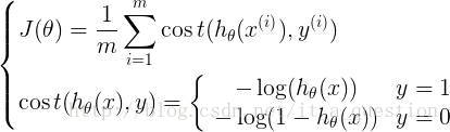
可以综合起来为：

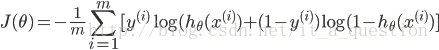
其中：

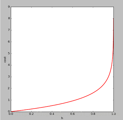
为什么不用线性回归的代价函数表示，因为线性回归的代价函数可能是非凸的，对于分类问题，使用梯度下降很难得到最小值，上面的代价函数是凸函数的图像如下，即y=1时：

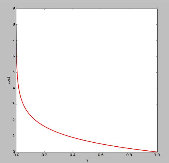
可以看出，当趋于1，y=1,与预测值一致，此时付出的代价cost趋于0，若趋于0，y=1,此时的代价cost值非常大，我们最终的目的是最小化代价值，同理的图像如下（y=0）：

2、梯度
同样对代价函数求偏导：

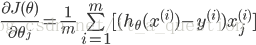
可以看出与线性回归的偏导数一致
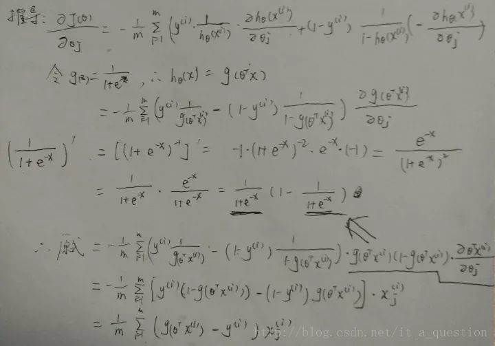
推导过程

3、正则化
目的是为了防止过拟合。在代价函数中加上一项

注意j是重1开始的，因为theta(0)为一个常数项，X中最前面一列会加上1列1，所以乘积还是theta(0),feature没有关系，没有必要正则化

正则化后的代价：

# 代价函数
def costFunction(initial_theta,X,y,inital_lambda):
    m = len(y)
    J = 0

    h = sigmoid(np.dot(X,initial_theta))    # 计算h(z)
    theta1 = initial_theta.copy()           # 因为正则化j=1从1开始，不包含0，所以复制一份，前theta(0)值为0 
    theta1[0] = 0   

    temp = np.dot(np.transpose(theta1),theta1)
    J = (-np.dot(np.transpose(y),np.log(h))-np.dot(np.transpose(1-y),np.log(1-h))+temp*inital_lambda/2)/m   # 正则化的代价方程
    return J

正则化后的代价的梯度

# 计算梯度 
def gradient(initial_theta,X,y,inital_lambda):
    m = len(y)
    grad = np.zeros((initial_theta.shape[0]))

    h = sigmoid(np.dot(X,initial_theta))# 计算h(z)
    theta1 = initial_theta.copy()
    theta1[0] = 0

    grad = np.dot(np.transpose(X),h-y)/m+inital_lambda/m*theta1 #正则化的梯度
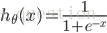
    return grad  

4、S型函数（即）

实现代码：

# S型函数
def sigmoid(z):
    h = np.zeros((len(z),1))    # 初始化，与z的长度一置

    h = 1.0/(1.0+np.exp(-z))    
    return h 

5、映射为多项式
因为数据的feture可能很少，导致偏差大，所以创造出一些feture结合
eg:映射为2次方的形式: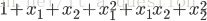
实现代码：

# 映射为多项式 
def mapFeature(X1,X2):
    degree = 3;                     # 映射的最高次方
    out = np.ones((X1.shape[0],1))  # 映射后的结果数组（取代X）
    '''
    这里以degree=2为例，映射为1,x1,x2,x1^2,x1,x2,x2^2
    '''
    for i in np.arange(1,degree+1): 
        for j in range(i+1):
            temp = X1**(i-j)*(X2**j)    #矩阵直接乘相当于matlab中的点乘.*
            out = np.hstack((out, temp.reshape(-1,1)))
    return out

6、使用scipy的优化方法
梯度下降使用scipy中optimize中的fmin_bfgs函数
调用scipy中的优化算法fmin_bfgs（拟牛顿法Broyden-Fletcher-Goldfarb-Shanno costFunction是自己实现的一个求代价的函数，
initial_theta表示初始化的值,
fprime指定costFunction的梯度
args是其余测参数，以元组的形式传入，最后会将最小化costFunction的theta返回

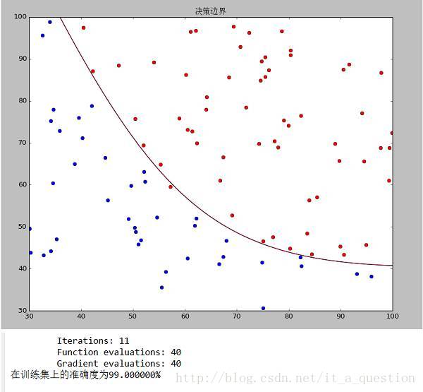
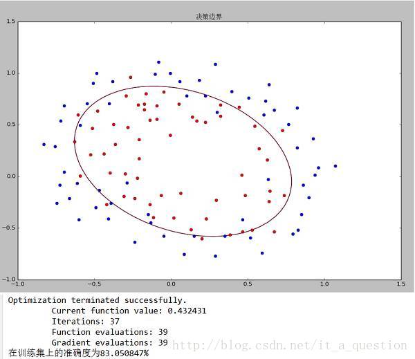
result = optimize.fmin_bfgs(costFunction, initial_theta, fprime=gradient, args=(X,y,initial_lambda))     

7、运行结果

data1决策边界和准确度

data2决策边界和准确度

8、使用scikit-learn库中的逻辑回归模型实现
https://github.com/lawlite19/MachineLearning_Python/blob/master/LogisticRegression/LogisticRegression_scikit-learn.py
导入包

from sklearn.linear_model import LogisticRegression 
from sklearn.preprocessing import StandardScaler 
from sklearn.cross_validation import train_test_split 
import numpy as np 

划分训练集和测试集

# 划分为训练集和测试集     
x_train,x_test,y_train,y_test = train_test_split(X,y,test_size=0.2) 

归一化

# 归一化     
scaler = StandardScaler()     
scaler.fit(x_train)     
x_train = scaler.fit_transform(x_train)     
x_test = scaler.fit_transform(x_test) 

逻辑回归

#逻辑回归     
model = LogisticRegression()     
model.fit(x_train,y_train) 

预测

# 预测     
predict = model.predict(x_test)    
right = sum(predict == y_test)          
predict = np.hstack((predict.reshape(-1,1),y_test.reshape(-1,1)))   # 将预测值和真实值放在一块，好观察     
print predict     
print ('测试集准确率：%f%%'%(right*100.0/predict.shape[0]))       #计算在测试集上的准确度 

逻辑回归_手写数字识别_OneVsAll

https://github.com/lawlite19/MachineLearning_Python/blob/master/LogisticRegression

全部代码
https://github.com/lawlite19/MachineLearning_Python/blob/master/LogisticRegression/LogisticRegression_OneVsAll.py
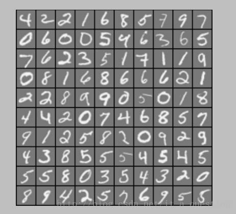
1、随机显示100个数字
我没有使用scikit-learn中的数据集，像素是20*20px，彩色图如下

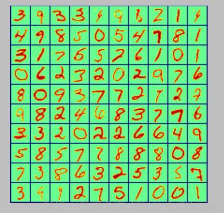
灰度图：

实现代码：

# 显示100个数字
def display_data(imgData):
    sum = 0
    '''
    显示100个数（若是一个一个绘制将会非常慢，可以将要画的数字整理好，放到一个矩阵中，显示这个矩阵即可）
    - 初始化一个二维数组
    - 将每行的数据调整成图像的矩阵，放进二维数组
    - 显示即可
    '''
    pad = 1
    display_array = -np.ones((pad+10*(20+pad),pad+10*(20+pad)))
    for i in range(10):
        for j in range(10):
            display_array[pad+i*(20+pad):pad+i*(20+pad)+20,pad+j*(20+pad):pad+j*(20+pad)+20] = (imgData[sum,:].reshape(20,20,order="F"))    # order=F指定以列优先，在matlab中是这样的，python中需要指定，默认以行
            sum += 1

    plt.imshow(display_array,cmap='gray')   #显示灰度图像
    plt.axis('off')
    plt.show()

2、OneVsAll
如何利用逻辑回归解决多分类的问题，OneVsAll就是把当前某一类看成一类，其他所有类别看作一类，这样有成了二分类的问题了。如下图，把途中的数据分成三类，先把红色的看成一类，把其他的看作另外一类，进行逻辑回归，然后把蓝色的看成一类，其他的再看成一类，以此类推…

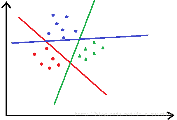
可以看出大于2类的情况下，有多少类就要进行多少次的逻辑回归分类

3、手写数字识别
共有0-9，10个数字，需要10次分类

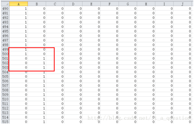
由于数据集y给出的是0,1,2…9的数字，而进行逻辑回归需要0/1的label标记，所以需要对y处理

说一下数据集，前500个是0,500-1000是1,…,所以如下图，处理后的y，前500行的第一列是1，其余都是0,500-1000行第二列是1，其余都是0….

然后调用梯度下降算法求解theta

实现代码：

# 求每个分类的theta，最后返回所有的all_theta    
def oneVsAll(X,y,num_labels,Lambda):
    # 初始化变量
    m,n = X.shape
    all_theta = np.zeros((n+1,num_labels))  # 每一列对应相应分类的theta,共10列
    X = np.hstack((np.ones((m,1)),X))       # X前补上一列1的偏置bias
    class_y = np.zeros((m,num_labels))      # 数据的y对应0-9，需要映射为0/1的关系
    initial_theta = np.zeros((n+1,1))       # 初始化一个分类的theta

    # 映射y
    for i in range(num_labels):
        class_y[:,i] = np.int32(y==i).reshape(1,-1) # 注意reshape(1,-1)才可以赋值

    #np.savetxt("class_y.csv", class_y[0:600,:], delimiter=',')    

    '''遍历每个分类，计算对应的theta值'''
    for i in range(num_labels):
        result = optimize.fmin_bfgs(costFunction, initial_theta, fprime=gradient, args=(X,class_y[:,i],Lambda)) # 调用梯度下降的优化方法
        all_theta[:,i] = result.reshape(1,-1)   # 放入all_theta中

    all_theta = np.transpose(all_theta) 
    return all_theta

4、预测

之前说过，预测的结果是一个概率值，利用学习出来的theta代入预测的S型函数中，每行的最大值就是是某个数字的最大概率，所在的列号就是预测的数字的真实值,因为在分类时，所有为0的将y映射在第一列，为1的映射在第二列，依次类推

实现代码：

# 预测
def predict_oneVsAll(all_theta,X):
    m = X.shape[0]
    num_labels = all_theta.shape[0]
    p = np.zeros((m,1))
    X = np.hstack((np.ones((m,1)),X))   #在X最前面加一列1

    h = sigmoid(np.dot(X,np.transpose(all_theta)))  #预测

    '''
    返回h中每一行最大值所在的列号
    - np.max(h, axis=1)返回h中每一行的最大值（是某个数字的最大概率）
    - 最后where找到的最大概率所在的列号（列号即是对应的数字）
    '''
    p = np.array(np.where(h[0,:] == np.max(h, axis=1)[0]))  
    for i in np.arange(1, m):
        t = np.array(np.where(h[i,:] == np.max(h, axis=1)[i]))
        p = np.vstack((p,t))
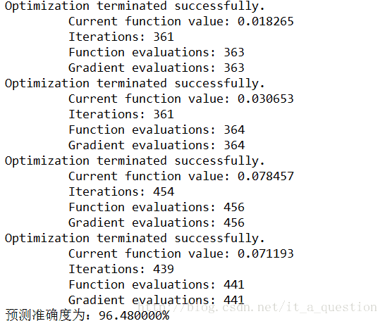
    return p

5、运行结果

10次分类，在训练集上的准确度：

6、使用scikit-learn库中的逻辑回归模型实现
https://github.com/lawlite19/MachineLearning_Python/blob/master/LogisticRegression/LogisticRegression_OneVsAll_scikit-learn.py

1、导入包

from scipy import io as spio 
import numpy as np 
from sklearn import svm 
from sklearn.linear_model import LogisticRegression 

2、加载数据

data = loadmat_data("data_digits.mat")      
X = data['X']   # 获取X数据，每一行对应一个数字20x20px     
y = data['y']   # 这里读取mat文件y的shape=(5000, 1)     
y = np.ravel(y) # 调用sklearn需要转化成一维的(5000,)

3、拟合模型

model = LogisticRegression()     
model.fit(X, y) # 拟合 

4、预测

predict = model.predict(X) #预测          
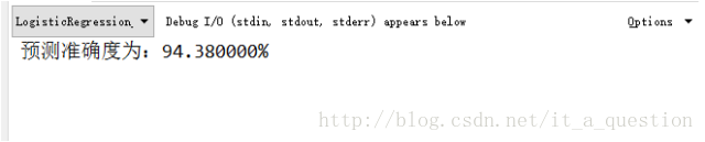
print u"预测准确度为：%f%%"%np.mean(np.float64(predict == y)*100) 

5、输出结果（在训练集上的准确度）