【Pytorch官方教程】从零开始自己搭建RNN1 - 字母级RNN的分类任务

本文链接：https://blog.csdn.net/iteapoy/article/details/106478462

文章目录

0 前言
1 数据与说明
- 数据下载
- 任务说明
2 基础原理
3 代码

0 前言

来自官方教程，对于萌新学习用Pytorch做NLP任务有很大的帮助，就翻译过来，顺便自己Mark一下，因为打开官网有时候太慢了，还是看自己写的Blog比较快。另外，之前在做⭐ 李宏毅2020机器学习作业4-RNN：句子情感分类的时候，代码看起来有些难度。之前的几个作业都还能看懂，但是作业4实在跳跃度太大了，就先拿这几个练个手。

这是官方教程中同一个系列的文章，总共有3篇：

第一篇，教你搭建一个字母级别（character-level）的RNN，对名字进行分类，是一个分类的任务。
第二篇，教你搭建一个字母级别（character-level）的RNN，生成名字，是一个自然语言生成的任务。
第三篇，教你搭建一个Seq2Seq的RNN，进行机器翻译，也是一个自然语言生成的任务。Seq2Seq是序列到序列的模型，类似于单词级别（word-level）的RNN。

博主更新完的本系列文章：

1 数据与说明

数据下载

数据下载链接：点击下载

数据是一个data.zip压缩包，解压后的目录树如下所示：

D:.
│  eng-fra.txt
│  
└─names
        Arabic.txt
        Chinese.txt
        Czech.txt
        Dutch.txt
        English.txt
        French.txt
        German.txt
        Greek.txt
        Irish.txt
        Italian.txt
        Japanese.txt
        Korean.txt
        Polish.txt
        Portuguese.txt
        Russian.txt
        Scottish.txt
        Spanish.txt
        Vietnamese.txt

eng-fra.txt 是第三篇翻译任务中要用到的，这次我们只用到 /name 这个文件夹下的18个文件，每个文件以语言命名，格式为：[Language].txt。打开后，里面是该语言中常用的姓/名。

比如：打开我们最熟悉的 Chinese.txt，可以看到每一行是一个姓或者名（有一些姓/名确实有点点奇怪，但整体来说问题不大）。

Ang
Au-Yong
Bai
Ban
Bao
Bei
Bian
Bui
Cai
Cao
Cen
……

任务说明

这次任务的目标是，输入一个姓名，根据它的拼写，用循环神经网络对它分类，判断它属于哪个语言里的姓名。

比如：

$ python predict.py Hinton
(-0.47) Scottish
(-1.52) English
(-3.57) Irish

$ python predict.py Schmidhuber
(-0.19) German
(-2.48) Czech
(-2.68) Dutch

Hinton 这个姓名很有可能是Scottish，其次可能是English，再其次可能是Irish。
Schmidhuber 这个姓名很有可能是German，其次可能是Czech，再其次可能是Dutch。

2 基础原理

RNN

在讲解代码前，我们简单回顾/了解一下循环神经网络。如果你已经了解，直接可以跳过。

一般的神经网络都是单向的，一层连着下一层。而循环神经网络（Recurrent Neural Network）和它的名字一样，里面引入了循环体结构，就像我们写代码的 for 或者 while 循环一样，某一步的循环体就像下面这样：

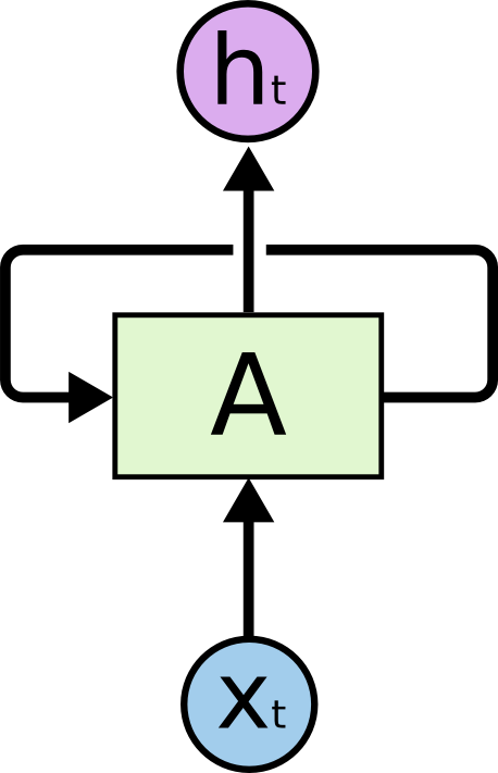
$x_t$ 是第 t 步循环时的输入， $h_t$ 是第 t 步循环的输出，它们都是向量，不是标量（一个数值）。这样一个循环体就可以把信息从上一步传递到下一步。不过，这样的循环体看起来不太好懂，让我们把它按时序展平（降维攻击！！！），变成一般的神经网络那样的单向传播结构。展开后就是一个链状结构：

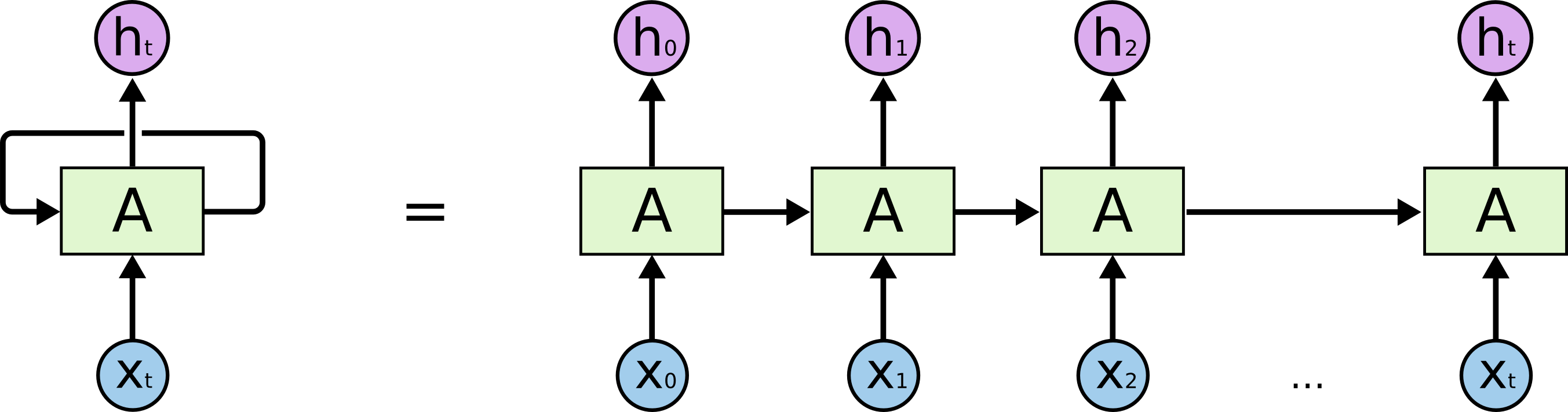
这样我们就可以看到，从第0步到第t步之间都发生了一些什么。每一个A块里的东西都是一样的，你可以理解成 for (i=0; i<t; i++) 或者 for i in range(t) 块中的代码。所以，我们只需要写某一步的变量更新方式，然后让它循环就可以了。

现在的问题是：变量到底应该怎么更新？输入的 $x_t$ 应该如何处理，才能变成输出的 $h_t$ ？图里的 A 内部具体的更新结构如下：

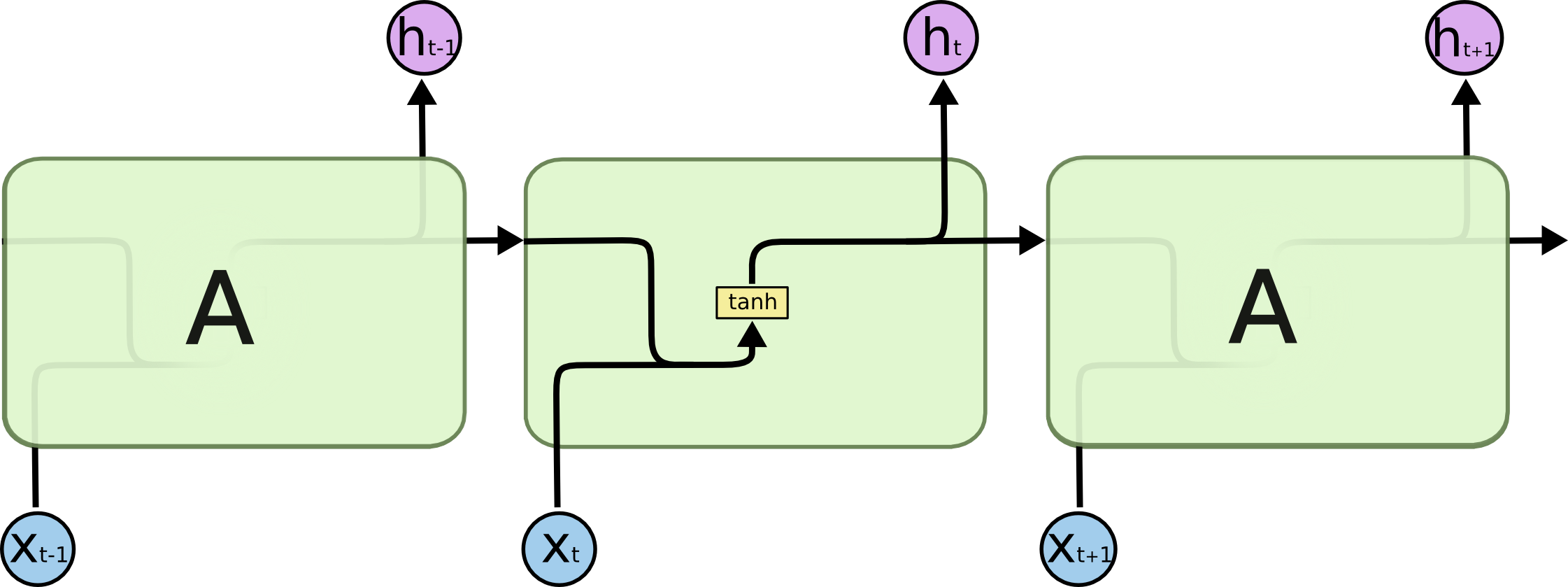
流程如下：

把上一步输出的 $h_{t-1}$ 乘上一个权重矩阵 $W_h$ ，变成 $W_hh_{t-1}$ 。h是隐藏层（hidden layer）的简写
这一步输入的 $x_t$ 也乘上一个权重矩阵 $W_i$ ，变成 $W_ix_{t}$ 。i是输入（input）的简写
把它们相加，变成 $W_hh_{t-1}+W_ix_{t}$
经过一个 $\tanh(·)$ 函数的处理，就得到了这一步的输出： $h_t = \tanh(W_hh_{t-1}+W_ix_{t})$

把流程1到流程4反复循环，就是一个最简单的RNN。

如果你看到了这里，恭喜你！你已经学会RNN了！

如果你还不会，我们再演示下一遍循环：

把上一步输出的 $h_{t}$ 乘上一个权重矩阵 $W_h$ ，变成 $W_hh_{t}$
这一步输入的 $x_{t+1}$ 也乘上一个权重矩阵 $W_i$ ，变成 $W_ix_{t+1}$
把它们相加，变成 $W_hh_{t}+W_ix_{t+1}$
经过一个 $\tanh(·)$ 函数的处理，就得到了这一步的输出： $h_{t+1} = \tanh(W_hh_{t}+W_ix_{t+1})$

你会发现，变化的只有 $h_{t}$ 和 $x_{t+1}$ ，它们的下标从 $t - 1$ 变成了 $t$ ，从 $t$ 变成了 $t + 1$ ，而 $W_h$ 和 $W_i$ 并没有与时间步 $t$ 相关的下标，始终只有这两个矩阵，当然，你在训练过程中，这两个矩阵中的数字会发生变化，因为它们是模型要学习的“参数”。

另外，你可能会看到一种带有偏置向量 $b$ 的更新方式：

$h_t = \tanh((W_hh_{t-1}+b_h)+(W_ix_{t}+b_i))$

我们这里进行了简化，即令所有的向量 $b$ 都为0。另外，我们在初始化向量 $h_0$ 的时候，也会把它初始化成全为0的向量。

RNN这样一个结构用来处理有前后关联的序列非常有效，因此在自然语言处理里也取得了不错的成绩。因为一句话可以看成是许多词组成的序列，这些词之前有前后文/上下文关系。

LSTM

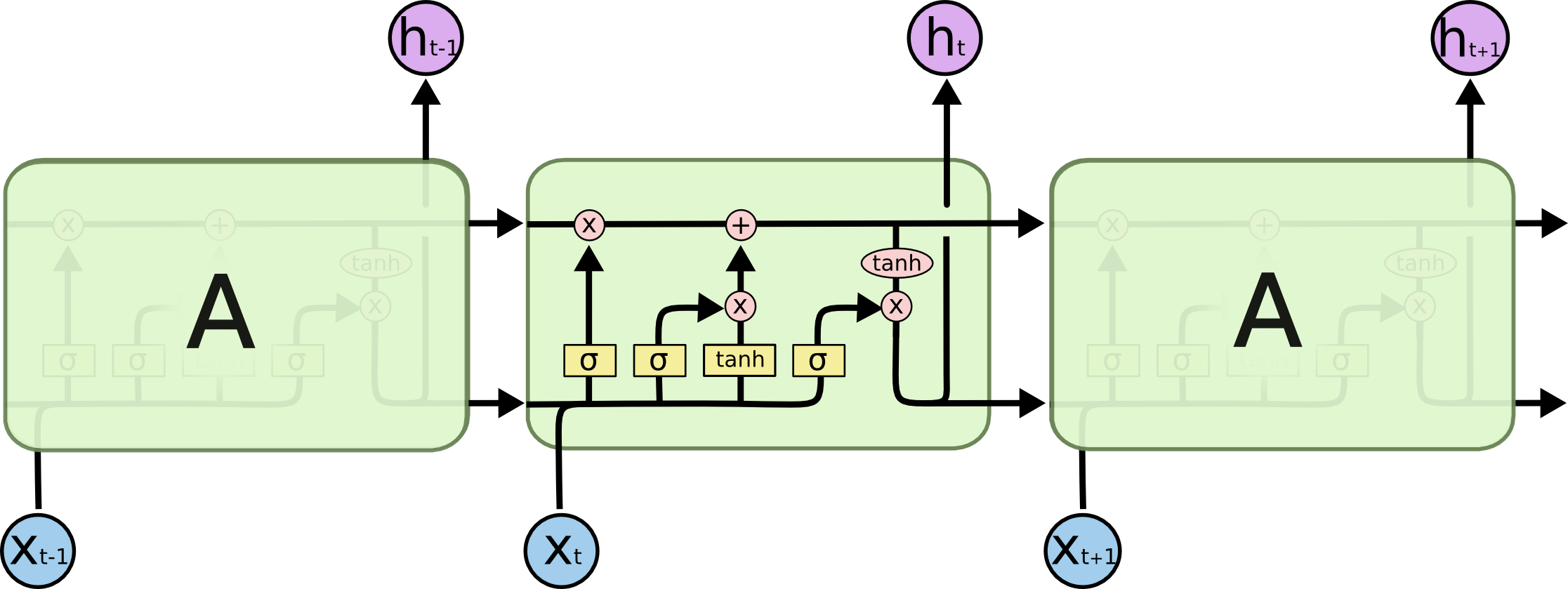
不过，普通的RNN有一个长短句依赖的问题（不细讲了，反正就是不太好使），所以有人提出了LSTM来改进RNN。LSTM是长短期记忆网络（LSTM，Long Short-Term Memory），通过三个门（遗忘门、输入门、输出门）的控制，存储短期记忆或长期记忆。它的整体流程还是这样：

但是，LSTM里的一个 A 内部的结构变成了这样子：

自从RNN整容成LSTM后，你再也不认识它了……

说实话，这张图美则美矣，我觉得还是李宏毅老师的简化版容易入门，一起贴上来吧！图里省略了几个 $\tanh(·)$ 函数，更方便理解：
在这里插入图片描述

图中是第 t 步的更新情况，就是 $\sigma(·)$ 的S型曲线，即sigmoid函数：

$\sigma(x)=\frac{1}{1+e^{-x}}$

画出来就长这样了：

我们先看李宏毅老师的高级简化版：

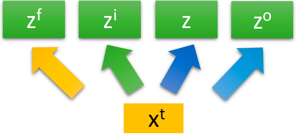
对同一个输入 $x_t$ ，乘上不同的权重 $W_f$ 、 $W_i$ 、 $W$ 、 $W_o$ 就变成了四个不同的值：

$z_f=W_fx_t$ ，是遗忘门（Forget Gate）的输入
$z_i=W_ix_t$ ，是输入门（Input Gate）的输入
$z=Wx_t$ ，是真正的输入（和输入门的输入是不一样的）
$z_o=W_ox_t$ ，是输出门（Output Gate）的输入

右边的图从下往上看，我们先来看 ~~红配绿~~ 红色方框圈出来的部分，输入和输入门的更新，它负责判断是否要接受新的输入：
在这里插入图片描述

$z_i$ 乘以权重 $W_i$ ，加上偏置向量 $b_i$ ，经过输入门，变成了 $i_t = \sigma(W_iz_i+b_i)$
$z$ 乘以权重 $W_c$ ，加上偏置向量 $b_c$ ，经过 $\tanh(·)$ ，变成了 $\tilde{c}_t=\sigma(W_cz+b_c)$ 。这里的 $c$ 是上面的cell的简写，它是一个存储单元
把 $i_t$ 和 $\tilde{c}_t$ 按元素相乘（Hadamard乘积，运算符为 $\odot$ 或 $*$ ），得到 $i_t*\tilde{c}_t$ ，然后输入cell

以上就这样完了。

Hadamard乘积：

假设输入矩阵 $A=\{a_{ij}\}$ ， $B=\{b_{ij}\}$ ，都是大小为 $m\times n$ 的矩阵，那么
$B=\left[\begin{array}{cccc} a_{11} b_{11} & a_{12} b_{12} & \cdots & a_{1 n} b_{1 n} \\ a_{21} b_{21} & a_{22} b_{22} & \cdots & a_{2 n} b_{2 n} \\ \vdots & \vdots & & \vdots \\ a_{m 1} b_{m 1} & a_{m 2} b_{m 2} & \cdots & a_{m n} b_{m n} \end{array}\right]$

然后，我们来看看蓝色圈出来的部分，是遗忘门的更新，它负责判断是否要更新cell中的值，如果更新了，就要忘记之前的值，写入新的值：
在这里插入图片描述

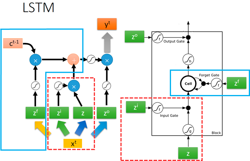
cell中存放了上一步的存储向量 $c_{t-1}$
$z_f$ 乘以权重 $W_f$ ，加上偏置向量 $b_f$ ，经过遗忘门，变成了 $f_t=\sigma(W_fz_f+b_f)$
在cell中，把 $c_{t-1}$ 和 $f_t$ 同样按元素相乘，然后和刚才提到的 $i_t*\tilde{c}_t$ 相加，就变成了新的存储向量 $c_t=c_{t-1}* f_t+i_t*\tilde{c}_t$

最后，我们来看一下橙色圈出来的部分，输出门的更新，它负责判断是否要输出最后的值：
在这里插入图片描述

新的 $c_t$ 先通过一个 $\tanh(·)$ 函数，变成 $tanh(c_t)$
$z_o$ 乘以权重 $W_o$ ，加上偏置向量 $b_o$ ，经过输出门，变成了 $o_t=\sigma(W_oz_o+b_o)$
把 $tanh(c_t)$ 和 $o_t$ 按元素相乘，得到新的隐藏层状态 $h_t=o_t*\tanh(c_t)$
隐藏层状态 $h_t$ 通过一个softmax函数，得到最后的输出 $y_t=softmax(h_t)$

以上，就是LSTM中某一步的状态更新情况。我们再回头看这张图：

之前， $z_f$ 、 $z_i$ 、 $z$ 、 $z_o$ 都是用 $x_t$ 乘以不同的权重得到的。但是，光凭 $x_t$ ，不足以传递足够多的信息，我们把 $x_t$ 和上一步输出的隐藏层状态 $h_{t-1}$ 拼在一起，变成一个新的输入向量 $x_t, h_{t-1}]$ 。上面的更新公式变成了下面这样：

在这里插入图片描述

说到这里，所谓的“门”，实际上就是一个 $\sigma(·)$ 或者 $\tanh(·)$ 函数。不过，一个好的命名更便于装X 形象化地理解。

因为 LSTM 实在比 RNN 优秀太多，所以我们一般称循环神经网络的时候，其实都是在说LSTM。

GRU

因为LSTM太复杂，而且容易过拟合，有一个简化版的LSTM，叫做GRU，它把遗忘门和输入门合并成了一个更新门，从三个门减少到了两个门，更新公式如下：
在这里插入图片描述
这里省略了偏置向量 $b$ 。

one-hot 编码

刚才说到，输入是 $x_t$ 。在自然语言处理中，我们不可能把一个字母作为输入，进行向量、矩阵的乘法，因此，我们需要把它变成一个特征向量。 $x_t$ 可以是字母的特征向量，或者单词的特征向量，或者句子的特征向量。

本文中， $x_t$ 是一个字母的特征向量。

我们知道，计算机存储字母一般是用ASCII编码，比如a是97，b是98，c是99，d是100……或者我们也可以说，a是1，b是2，c是3……但是，用这样的连续值表示字母，有一个问题，这意味着 a 和 b 的关系比较近，a 和 z 的关系比较远。虽然 a 和 z 在字母表里确实隔得比较远，但是实际上，它们并没有这种内在的关系。我们用一种编码表示它们的时候，它们应该是相互独立的，即对它们进行离散化。

我们通常用到的是 one-hot 编码。它是一个长度为 $n$ 的向量，只有 $1$ 个数字是1，其它的 $n - 1$ 个数字都是0。one-hot 编码使得每个字母在它们各自的维度上，与其它字母是独立的。

比如一个单词 “apple”，就分别对a、p、p、l、e 编码，作为输入，LSTM需要循环5次。

$x_0 = [1,0,0,0,0\ldots,0,0]$ : a
$x_1 = [0,1,0,0,0\ldots,0,0]$ : p
$x_2 = [0,1,0,0,0\ldots,0,0]$ : p
$x_3 = [0,0,1,0,0\ldots,0,0]$ : l
$x_4 = [0,0,0,1,0\ldots,0,0]$ : e

上面就是本文提到的字母级（character-level）RNN，而单词级（word-level）RNN就是把整个单词 “apple” 编码成一个向量。通常，对单词的编码用于Seq2Seq模型，即处理的是一个序列 “An apple a day keeps the doctor away”：

$x_0 = [1,0,0,0,0,0,0,0,\ldots,0,0]$ : an
$x_1 = [0,1,0,0,0,0,0,0,\ldots,0,0]$ : apple
$x_2 = [0,0,1,0,0,0,0,0,\ldots,0,0]$ : a
$x_3 = [0,0,0,1,0,0,0,0,\ldots,0,0]$ : day
$x_4 = [0,0,0,0,1,0,0,0,\ldots,0,0]$ : keeps
$x_5 = [0,0,0,0,0,1,0,0,\ldots,0,0]$ : the
$x_6 = [0,0,0,0,0,0,1,0\ldots,0,0]$ : doctor
$x_7 = [0,0,0,0,0,0,0,1\ldots,0,0]$ : away

不过，本文中， $x_t$ 是一个字母的特征向量，而不是一个单词的特征向量。

3 代码

数据预处理

首先，我们把所有的 /name/[Language].txt 文件读进来。

n_letters 表示所有字母的数量。因为某些语言的字母和常见的英文字母不太一样，所以我们需要把它转化成普普通通的英文字母，用到了 unicodeToAscii() 函数。

from __future__ import unicode_literals,print_function,division
from io import open
import glob
import os

def findFiles(path): return glob.glob(path)

print(findFiles('data/names/*.txt'))

import unicodedata
import string

all_letters = string.ascii_letters + " .,;'"
n_letters = len(all_letters)

def unicodeToAscii(s):
    return ''.join(
      c for c in unicodedata.normalize('NFD',s)
      if unicodedata.category(c)!='Mn'
      and c in all_letters
    )

print(unicodeToAscii('Ślusàrski'))

Out:

['data/names/Greek.txt', 'data/names/Dutch.txt', 'data/names/Irish.txt', 'data/names/Arabic.txt', 'data/names/Korean.txt', 'data/names/French.txt', 'data/names/Spanish.txt', 'data/names/German.txt', 'data/names/Portuguese.txt', 'data/names/Italian.txt', 'data/names/Vietnamese.txt', 'data/names/Russian.txt', 'data/names/Scottish.txt', 'data/names/Chinese.txt', 'data/names/English.txt', 'data/names/Japanese.txt', 'data/names/Czech.txt', 'data/names/Polish.txt']
Slusarski

文件 [Language].txt 的命名中，Language 就是类别 category 。把每个文件打开，读入每一行，放入一个数组 lines = [names ...] 。建立一个词典 category_lines = {language: lines}

category_lines = {}
all_categories = []

def readLines(filename):
    lines = open(filename,encoding='utf-8').read().strip().split('\n')
    return [unicodeToAscii(line) for line in lines]

for filename in findFiles('data/names/*.txt'):
    category = os.path.splitext(os.path.basename(filename))[0]
    all_categories.append(category)
    lines = readLines(filename)
    category_lines[category] = lines

n_categories = len(all_categories)
print(all_categories)
print(category_lines['Italian'])

Out:

['Greek', 'Dutch', 'Irish', 'Arabic', 'Korean', 'French', 'Spanish', 'German', 'Portuguese', 'Italian', 'Vietnamese', 'Russian', 'Scottish', 'Chinese', 'English', 'Japanese', 'Czech', 'Polish']
['Abandonato', 'Abatangelo', 'Abatantuono', 'Abate', 'Abategiovanni', 'Abatescianni', 'Abba', 'Abbadelli', 'Abbascia', 'Abbatangelo', 'Abbatantuono', 'Abbate', 'Abbatelli', 'Abbaticchio', 'Abbiati', 'Abbracciabene', 'Abbracciabeni', 'Abelli', 'Abello', 'Abrami', 'Abramo', 'Acardi', 'Accardi', 'Accardo', 'Acciai', 'Acciaio', 'Acciaioli', 'Acconci', 'Acconcio', 'Accorsi', 'Accorso', 'Accosi', 'Accursio', 'Acerbi', 'Acone', 'Aconi', 'Acqua', 'Acquafredda', 'Acquarone', 'Acquati', 'Adalardi', 'Adami', 'Adamo', 'Adamoli', 'Addario', 'Adelardi', 'Adessi', 'Adimari', 'Adriatico', 'Affini', 'Africani', 'Africano', 'Agani', 'Aggi', 'Aggio', 'Agli', 'Agnelli', 'Agnellutti', 'Agnusdei', 'Agosti', 'Agostini', 'Agresta', 'Agrioli', 'Aiello', 'Aiolfi', 'Airaldi', 'Airo', 'Aita', 'Ajello', 'Alagona', 'Alamanni', 'Albanesi', 'Albani', 'Albano', 'Alberghi', 'Alberghini', 'Alberici', 'Alberighi', 'Albero', 'Albini', 'Albricci', 'Albrici', 'Alcheri', 'Aldebrandi', 'Alderisi', 'Alduino', 'Alemagna', 'Aleppo', 'Alesci', 'Alescio', 'Alesi', 'Alesini', 'Alesio', 'Alessandri', 'Alessi', 'Alfero', 'Aliberti', 'Alinari', 'Aliprandi', 'Allegri', 'Allegro', 'Alo', 'Aloia', 'Aloisi', 'Altamura', 'Altimari', 'Altoviti', 'Alunni', 'Amadei', 'Amadori', 'Amalberti', 'Amantea', 'Amato', 'Amatore', 'Ambrogi', 'Ambrosi', 'Amello', 'Amerighi', 'Amoretto', 'Angioli', 'Ansaldi', 'Anselmetti', 'Anselmi', 'Antonelli', 'Antonini', 'Antonino', 'Aquila', 'Aquino', 'Arbore', 'Ardiccioni', 'Ardizzone', 'Ardovini', 'Arena', 'Aringheri', 'Arlotti', 'Armani', 'Armati', 'Armonni', 'Arnolfi', 'Arnoni', 'Arrighetti', 'Arrighi', 'Arrigucci', 'Aucciello', 'Azzara', 'Baggi', 'Baggio', 'Baglio', 'Bagni', 'Bagnoli', 'Balboni', 'Baldi', 'Baldini', 'Baldinotti', 'Baldovini', 'Bandini', 'Bandoni', 'Barbieri', 'Barone', 'Barsetti', 'Bartalotti', 'Bartolomei', 'Bartolomeo', 'Barzetti', 'Basile', 'Bassanelli', 'Bassani', 'Bassi', 'Basso', 'Basurto', 'Battaglia', 'Bazzoli', 'Bellandi', 'Bellandini', 'Bellincioni', 'Bellini', 'Bello', 'Bellomi', 'Belloni', 'Belluomi', 'Belmonte', 'Bencivenni', 'Benedetti', 'Benenati', 'Benetton', 'Benini', 'Benivieni', 'Benvenuti', 'Berardi', 'Bergamaschi', 'Berti', 'Bertolini', 'Biancardi', 'Bianchi', 'Bicchieri', 'Biondi', 'Biondo', 'Boerio', 'Bologna', 'Bondesan', 'Bonomo', 'Borghi', 'Borgnino', 'Borgogni', 'Bosco', 'Bove', 'Bover', 'Boveri', 'Brambani', 'Brambilla', 'Breda', 'Brioschi', 'Brivio', 'Brunetti', 'Bruno', 'Buffone', 'Bulgarelli', 'Bulgari', 'Buonarroti', 'Busto', 'Caiazzo', 'Caito', 'Caivano', 'Calabrese', 'Calligaris', 'Campana', 'Campo', 'Cantu', 'Capello', 'Capello', 'Capello', 'Capitani', 'Carbone', 'Carboni', 'Carideo', 'Carlevaro', 'Caro', 'Carracci', 'Carrara', 'Caruso', 'Cassano', 'Castro', 'Catalano', 'Cattaneo', 'Cavalcante', 'Cavallo', 'Cingolani', 'Cino', 'Cipriani', 'Cisternino', 'Coiro', 'Cola', 'Colombera', 'Colombo', 'Columbo', 'Como', 'Como', 'Confortola', 'Conti', 'Corna', 'Corti', 'Corvi', 'Costa', 'Costantini', 'Costanzo', 'Cracchiolo', 'Cremaschi', 'Cremona', 'Cremonesi', 'Crespo', 'Croce', 'Crocetti', 'Cucinotta', 'Cuocco', 'Cuoco', "D'ambrosio", 'Damiani', "D'amore", "D'angelo", "D'antonio", 'De angelis', 'De campo', 'De felice', 'De filippis', 'De fiore', 'De laurentis', 'De luca', 'De palma', 'De rege', 'De santis', 'De vitis', 'Di antonio', 'Di caprio', 'Di mercurio', 'Dinapoli', 'Dioli', 'Di pasqua', 'Di pietro', 'Di stefano', 'Donati', "D'onofrio", 'Drago', 'Durante', 'Elena', 'Episcopo', 'Ermacora', 'Esposito', 'Evangelista', 'Fabbri', 'Fabbro', 'Falco', 'Faraldo', 'Farina', 'Farro', 'Fattore', 'Fausti', 'Fava', 'Favero', 'Fermi', 'Ferrara', 'Ferrari', 'Ferraro', 'Ferrero', 'Ferro', 'Fierro', 'Filippi', 'Fini', 'Fiore', 'Fiscella', 'Fiscella', 'Fonda', 'Fontana', 'Fortunato', 'Franco', 'Franzese', 'Furlan', 'Gabrielli', 'Gagliardi', 'Gallo', 'Ganza', 'Garfagnini', 'Garofalo', 'Gaspari', 'Gatti', 'Genovese', 'Gentile', 'Germano', 'Giannino', 'Gimondi', 'Giordano', 'Gismondi', 'Giugovaz', 'Giunta', 'Goretti', 'Gori', 'Greco', 'Grillo', 'Grimaldi', 'Gronchi', 'Guarneri', 'Guerra', 'Guerriero', 'Guidi', 'Guttuso', 'Idoni', 'Innocenti', 'Labriola', 'Laconi', 'Lagana', 'Lagomarsino', 'Lagorio', 'Laguardia', 'Lama', 'Lamberti', 'Lamon', 'Landi', 'Lando', 'Landolfi', 'Laterza', 'Laurito', 'Lazzari', 'Lecce', 'Leccese', 'Leggieri', 'Lemmi', 'Leone', 'Leoni', 'Lippi', 'Locatelli', 'Lombardi', 'Longo', 'Lupo', 'Luzzatto', 'Maestri', 'Magro', 'Mancini', 'Manco', 'Mancuso', 'Manfredi', 'Manfredonia', 'Mantovani', 'Marchegiano', 'Marchesi', 'Marchetti', 'Marchioni', 'Marconi', 'Mari', 'Maria', 'Mariani', 'Marino', 'Marmo', 'Martelli', 'Martinelli', 'Masi', 'Masin', 'Mazza', 'Merlo', 'Messana', 'Micheli', 'Milani', 'Milano', 'Modugno', 'Mondadori', 'Mondo', 'Montagna', 'Montana', 'Montanari', 'Monte', 'Monti', 'Morandi', 'Morello', 'Moretti', 'Morra', 'Moschella', 'Mosconi', 'Motta', 'Muggia', 'Muraro', 'Murgia', 'Murtas', 'Nacar', 'Naggi', 'Naggia', 'Naldi', 'Nana', 'Nani', 'Nanni', 'Nannini', 'Napoleoni', 'Napoletani', 'Napoliello', 'Nardi', 'Nardo', 'Nardovino', 'Nasato', 'Nascimbene', 'Nascimbeni', 'Natale', 'Nave', 'Nazario', 'Necchi', 'Negri', 'Negrini', 'Nelli', 'Nenci', 'Nepi', 'Neri', 'Neroni', 'Nervetti', 'Nervi', 'Nespola', 'Nicastro', 'Nicchi', 'Nicodemo', 'Nicolai', 'Nicolosi', 'Nicosia', 'Nicotera', 'Nieddu', 'Nieri', 'Nigro', 'Nisi', 'Nizzola', 'Noschese', 'Notaro', 'Notoriano', 'Oberti', 'Oberto', 'Ongaro', 'Orlando', 'Orsini', 'Pace', 'Padovan', 'Padovano', 'Pagani', 'Pagano', 'Palladino', 'Palmisano', 'Palumbo', 'Panzavecchia', 'Parisi', 'Parma', 'Parodi', 'Parri', 'Parrino', 'Passerini', 'Pastore', 'Paternoster', 'Pavesi', 'Pavone', 'Pavoni', 'Pecora', 'Pedrotti', 'Pellegrino', 'Perugia', 'Pesaresi', 'Pesaro', 'Pesce', 'Petri', 'Pherigo', 'Piazza', 'Piccirillo', 'Piccoli', 'Pierno', 'Pietri', 'Pini', 'Piovene', 'Piraino', 'Pisani', 'Pittaluga', 'Poggi', 'Poggio', 'Poletti', 'Pontecorvo', 'Portelli', 'Porto', 'Portoghese', 'Potenza', 'Pozzi', 'Profeta', 'Prosdocimi', 'Provenza', 'Provenzano', 'Pugliese', 'Quaranta', 'Quattrocchi', 'Ragno', 'Raimondi', 'Rais', 'Rana', 'Raneri', 'Rao', 'Rapallino', 'Ratti', 'Ravenna', 'Re', 'Ricchetti', 'Ricci', 'Riggi', 'Righi', 'Rinaldi', 'Riva', 'Rizzo', 'Robustelli', 'Rocca', 'Rocchi', 'Rocco', 'Roma', 'Roma', 'Romagna', 'Romagnoli', 'Romano', 'Romano', 'Romero', 'Roncalli', 'Ronchi', 'Rosa', 'Rossi', 'Rossini', 'Rotolo', 'Rovigatti', 'Ruggeri', 'Russo', 'Rustici', 'Ruzzier', 'Sabbadin', 'Sacco', 'Sala', 'Salomon', 'Salucci', 'Salvaggi', 'Salvai', 'Salvail', 'Salvatici', 'Salvay', 'Sanna', 'Sansone', 'Santini', 'Santoro', 'Sapienti', 'Sarno', 'Sarti', 'Sartini', 'Sarto', 'Savona', 'Scarpa', 'Scarsi', 'Scavo', 'Sciacca', 'Sciacchitano', 'Sciarra', 'Scordato', 'Scotti', 'Scutese', 'Sebastiani', 'Sebastino', 'Segreti', 'Selmone', 'Selvaggio', 'Serafin', 'Serafini', 'Serpico', 'Sessa', 'Sgro', 'Siena', 'Silvestri', 'Sinagra', 'Sinagra', 'Soldati', 'Somma', 'Sordi', 'Soriano', 'Sorrentino', 'Spada', 'Spano', 'Sparacello', 'Speziale', 'Spini', 'Stabile', 'Stablum', 'Stilo', 'Sultana', 'Tafani', 'Tamaro', 'Tamboia', 'Tanzi', 'Tarantino', 'Taverna', 'Tedesco', 'Terranova', 'Terzi', 'Tessaro', 'Testa', 'Tiraboschi', 'Tivoli', 'Todaro', 'Toloni', 'Tornincasa', 'Toselli', 'Tosetti', 'Tosi', 'Tosto', 'Trapani', 'Traversa', 'Traversi', 'Traversini', 'Traverso', 'Trucco', 'Trudu', 'Tumicelli', 'Turati', 'Turchi', 'Uberti', 'Uccello', 'Uggeri', 'Ughi', 'Ungaretti', 'Ungaro', 'Vacca', 'Vaccaro', 'Valenti', 'Valentini', 'Valerio', 'Varano', 'Ventimiglia', 'Ventura', 'Verona', 'Veronesi', 'Vescovi', 'Vespa', 'Vestri', 'Vicario', 'Vico', 'Vigo', 'Villa', 'Vinci', 'Vinci', 'Viola', 'Vitali', 'Viteri', 'Voltolini', 'Zambrano', 'Zanetti', 'Zangari', 'Zappa', 'Zeni', 'Zini', 'Zino', 'Zunino']

接下来，就是要对字母进行one-hot编码，转成 tensor。

假设字母表中的字母数量为 n_letters ，一个字母的向量就是 < 1 × n_letters > 维，只有 1 个维度是1，其他 n_letters-1 维是0。

一个长度为 line_length 的单词，它的向量维度是 < line_length × n_letters > 维。

在机器学习中，通常我们会按照 batch 来训练，所以这里设定一个单词的 batch 是1，单词的向量维度变成了 < line_length × 1 × n_letters >

import torch

device = torch.device("cuda:0" if torch.cuda.is_available() else "cpu")

# 返回字母 letter 的索引 index
def letterToIndex(letter):
    return all_letters.find(letter)
  
# 把一个字母编码成tensor
def letterToTensor(letter):
    tensor = torch.zeros(1,n_letters)
    # 把字母 letter 的索引设定为1，其它都是0
    tensor[0][letterToIndex(letter)] = 1
    return tensor.to(device)

# 把一个单词编码成tensor
def lineToTensor(line):
    tensor = torch.zeros(len(line),1,n_letters)
    # 遍历单词中的所有字母，对每个字母 letter 它的索引设定为1，其它都是0
    for li, letter in enumerate(line):
        tensor[li][0][letterToIndex(letter)] = 1
    return tensor.to(device)

print(letterToTensor('J'))
print(lineToTensor('Jones').size())

Out:

tensor([[0., 0., 0., 0., 0., 0., 0., 0., 0., 0., 0., 0., 0., 0., 0., 0., 0., 0.,
         0., 0., 0., 0., 0., 0., 0., 0., 0., 0., 0., 0., 0., 0., 0., 0., 0., 1.,
         0., 0., 0., 0., 0., 0., 0., 0., 0., 0., 0., 0., 0., 0., 0., 0., 0., 0.,
         0., 0., 0.]], device='cuda:0')
torch.Size([5, 1, 57])

模型搭建

然后就是我们的模型部分，一个最普通的RNN。

它是一个两层的结构，i2h是输入 $x_t$ 到隐藏层 $h_t$ ，i2o是输入 $x_t$ 到输出 $o_t$ ，softmax是把输出 $o_t$ 变成预测值 $y_t$ 。实际上，它在这里是一个 LogSoftmax 函数，对应的损失函数是NLLLoss()，而如果它是一般的 Softmax 函数，对应的损失函数就是交叉熵损失 CrossEntropy() = Log (NLLLoss())。

这里设定隐藏层的向量维度为128维，为了简单，可以说是隐藏层的大小是128维。

模型真正的运行步骤在 forward()函数中，它的输入 input 即为 $x_t$ ，隐藏层hidden 即为 $h_t$ ：

combined = torch.cat((input,hidden),1)：把 $x_t$ 和上一步的 $h_{t-1}$ 拼接在一起，变成 $x_t, h_{t-1}]$
hidden = self.i2h(combined)：我们之前说，把输入 $x_t, h_{t-1}]$ 乘上权重 $W_h$ 变成新的隐藏层 $h_t = W_h[ x_t, h_{t-1}]$ ，这里实际上就是通过一个线性的全连接层 i2h，它的输入大小是 input_size + hidden_size，输出大小是 hidden_size
output = self.i2o(combined)：把输入 $x_t, h_{t-1}]$ 乘上权重 $W_o$ ，得到输出 $o_t = W_o[ x_t, h_{t-1}]$ ，同样是通过一个线性的全连接层 i2o，它的输入大小是 input_size + hidden_size，输出大小是 output_size
output = self.softmax(output)：通过一个softmax函数，把输出 $o_t$ 变成预测值 $y_t = \log softmax(o_t)$

import torch.nn as nn

class RNN(nn.Module):
    # 初始化定义每一层的输入大小，输出大小
    def __init__(self, input_size, hidden_size, output_size):
        super(RNN,self).__init__()

        self.hidden_size = hidden_size
        self.i2h = nn.Linear(input_size + hidden_size, hidden_size)
        self.i2o = nn.Linear(input_size + hidden_size, output_size)
        self.softmax = nn.LogSoftmax(dim=1)

    # 前向传播过程
    def forward(self, input, hidden):
        combined = torch.cat((input,hidden),1) 
        hidden = self.i2h(combined)
        output = self.i2o(combined)
        output = self.softmax(output)
        return output, hidden

    # 初始化隐藏层状态 h0  
    def initHidden(self):
        return torch.zeros(1,self.hidden_size).to(device)

n_hidden = 128
rnn = RNN(n_letters, n_hidden, n_categories)
rnn = rnn.to(device)

输入一个字母 A 测试一下：

input = letterToTensor('A')
hidden =torch.zeros(1, n_hidden).to(device)

output, next_hidden = rnn(input, hidden)
print(output)

Out:

tensor([[-2.8972, -2.8574, -2.9266, -2.9602, -2.9735, -3.0286, -2.9190, -2.7779,
         -2.8833, -2.8667, -2.9404, -2.8011, -2.8216, -2.8422, -2.8119, -2.8525,
         -2.9453, -2.9611]], device='cuda:0', grad_fn=<LogSoftmaxBackward>)

再输入名字 Albert 的第一个字母 A 测试一下：

input = lineToTensor('Albert')
hidden = torch.zeros(1, n_hidden).to(device)

output, next_hidden = rnn(input[0], hidden)
print(output)

Out:

tensor([[-2.8972, -2.8574, -2.9266, -2.9602, -2.9735, -3.0286, -2.9190, -2.7779,
         -2.8833, -2.8667, -2.9404, -2.8011, -2.8216, -2.8422, -2.8119, -2.8525,
         -2.9453, -2.9611]], device='cuda:0', grad_fn=<LogSoftmaxBackward>)

定义一个函数 categoryFromOutput() 可以把 $y_t$ 变成对应的类别。用 Tensor.topk 选出18个概率中，概率最大的那个的下标 category_i ，就是 $y_t$ 的类别。

def categoryFromOutput(output):
    top_n, top_i = output.topk(1)
    category_i = top_i[0].item()
    return all_categories[category_i], category_i

print(categoryFromOutput(output))

Out:

('German', 7)

训练

因为目前模型还没有被训练，所以上面的概率可以认为是随机产生的。接下来，我们要训练模型。这个教程里不是把所有的数据都拿来训练，而是随机采样一部分数据来训练。

用 randomChoice() 从所有数据中随机采样，先采样得到类别category，再从类别category中随机采样，得到姓名line。

randomTrainingExample() 将采样得到的 category-line对变成tensor。

import random

def randomChoice(l):
    return l[random.randint(0,len(l)-1)]

def randomTrainingExample():
    category = randomChoice(all_categories)
    line = randomChoice(category_lines[category])
    category_tensor = torch.tensor([all_categories.index(category)], dtype=torch.long).to(device)
    line_tensor = lineToTensor(line)
    return category, line, category_tensor, line_tensor

for i in range(10):
    category, line, category_tensor, line_tensor = randomTrainingExample()
    print('category = ', category, '/ line = ', line)

看看随机采样10个样本的情况：

Out:

category =  Scottish / line =  Mckenzie
category =  Irish / line =  Cormac
category =  German / line =  Farber
category =  French / line =  David
category =  Russian / line =  Yanaslov
category =  Korean / line =  Gwang 
category =  Chinese / line =  Hiu
category =  Russian / line =  Turchak
category =  Portuguese / line =  Madeira
category =  Spanish / line =  Castillo

定义损失函数为 NLLLoss()，学习率0.005。

在训练的每个循环会执行以下过程：

创建输入tensor和目标tensor
初始化隐藏层状态 $h_0$
输入每个字母 $x_t$ 并且
保存下一个字母需要的隐藏层状态 $h_t$
将模型预测的输出 $y_t$ 和目标 $y^*_t$ 之间进行对比
梯度反向传播
返回输出和损失函数

criterion = nn.NLLLoss()
learning_rate = 0.005

def train(category_tensor, line_tensor):
    hidden = rnn.initHidden()

    rnn.zero_grad()
    
    # RNN的循环
    for i in range(line_tensor.size()[0]):
        output, hidden = rnn(line_tensor[i],hidden)

    loss = criterion(output, category_tensor)
    loss.backward()

    # 更新参数
    for p in rnn.parameters():
        p.data.add_(p.grad.data, alpha=-learning_rate)

    return output, loss.item()

下面正式开始训练模型。

timeSince() 可以计算出训练时间。总共训练n_iters次，每次用1个样本作为训练。每 print_every 次打印当前的训练损失，每 plot_every 次把损失保存到 all_losses 数组中，便于之后画图。

import time
import math

n_iters = 100000
print_every = 5000
plot_every = 1000

current_loss = 0
all_losses = []

def timeSince(since):
    now = time.time()
    s = now-since
    return '%dm %ds'%(s//60,s%60)

start = time.time()

for iter in range(1, n_iters + 1):
    category, line, category_tensor, line_tensor = randomTrainingExample()
    output, loss = train(category_tensor, line_tensor)
    current_loss += loss

    if iter % print_every == 0:
        guess, guess_i = categoryFromOutput(output)
        correct = '√' if guess==category else '×(%s)'%category
        print('%d %d%% (%s) %.4f %s / %s %s' % 
          (iter, iter/n_iters*100,timeSince(start),loss,line,guess,correct))

    if iter % plot_every == 0:
        all_losses.append(current_loss/plot_every)
        current_loss = 0

Out:

5000 5% (0m 37s) 2.6348 Awdyukoff / English ×(Russian)
10000 10% (1m 14s) 1.2936 Dong / Vietnamese ×(Chinese)
15000 15% (1m 50s) 2.5938 Peij / Korean ×(Dutch)
20000 20% (2m 27s) 0.9246 Kwang  / Korean √
25000 25% (3m 3s) 0.7240 Echeverria / Spanish √
30000 30% (3m 39s) 2.3746 Benn / Chinese ×(German)
35000 35% (4m 16s) 3.1926 Wright / English ×(Scottish)
40000 40% (4m 53s) 1.5385 Vodden / Dutch ×(English)
45000 45% (5m 30s) 2.7799 Pander / German ×(Dutch)
50000 50% (6m 8s) 1.6615 Beckert / Dutch ×(German)
55000 55% (6m 46s) 0.4871 Mcdonald / Scottish √
60000 60% (7m 24s) 2.0091 Glenn / Scottish ×(English)
65000 65% (8m 2s) 1.5405 Flater / German √
70000 70% (8m 38s) 3.4448 Navara / Spanish ×(Czech)
75000 75% (9m 13s) 2.4132 Poulin / Russian ×(French)
80000 80% (9m 48s) 1.0501 Cao / Chinese ×(Vietnamese)
85000 85% (10m 22s) 1.1398 Sung / Chinese ×(Korean)
90000 90% (10m 57s) 2.2497 Frankland / Polish ×(English)
95000 95% (11m 32s) 1.3177 Williamson / Scottish √
100000 100% (12m 7s) 0.5656 Said / Arabic √

画图

画出损失函数随着训练的变化情况：

import matplotlib.pyplot as plt
import matplotlib.ticker as ticker

plt.figure()
plt.plot(all_losses)

在这里插入图片描述

为了看看模型在各个分类上的预测情况，我们要画出18国语言的混淆矩阵。每一行是真实的语言，每一列是预测的语言。用函数 evaluate() 来计算混淆矩阵。evaluate()和 train()非常相似，但是不需要梯度反向传播。

confusion = torch.zeros(n_categories, n_categories)
n_confusion = 10000

def evaluate(line_tensor):
    hidden = rnn.initHidden()

    for i in range(line_tensor.size()[0]):
        output, hidden = rnn(line_tensor[i],hidden)

    return output

for i in range(n_confusion):
    category, line, category_tensor,line_tensor = randomTrainingExample()
    output = evaluate(line_tensor)
    guess, guess_i = categoryFromOutput(output)
    category_i = all_categories.index(category)
    confusion[category_i][guess_i] += 1

for i in range(n_categories):
    confusion[i] = confusion[i] / confusion[i].sum()

fig = plt.figure()
ax = fig.add_subplot(111)
cax = ax.matshow(confusion.numpy())
fig.colorbar(cax)

ax.set_xticklabels(['']+all_categories,rotation=90)
ax.set_yticklabels(['']+all_categories)

ax.xaxis.set_major_locator(ticker.MultipleLocator(1))
ax.yaxis.set_major_locator(ticker.MultipleLocator(1))

plt.show()

在这里插入图片描述
两种语言连线处的正方形颜色越偏向暖色，表示两种语言的姓名越相似。从图中可以看到，有一些比较容易混淆语言，比如Chinese和Korean，还有Chinese和Vietnamese，English和Scottish。

预测

对于每个名字 input_line ，每次预测 n_predictions=3 个最有可能的类别，并且输出它们对应的概率：

def predict(input_line, n_predictions=3):
    print('\n> %s'%input_line)
    with torch.no_grad():
        output = evaluate(lineToTensor(input_line))

        topv, topi = output.topk(n_predictions,1,True)
        predictions = []

        for i in range(n_predictions):
            value = topv[0][i].item()
            category_index = topi[0][i].item()
            print('(%.2f) %s' % (value, all_categories[category_index]))
            predictions.append([value, all_categories[category_index]])

predict('Dovesky')
predict('Jackson')
predict('Satoshi')

Out:

> Dovesky
(-0.41) Russian
(-1.33) Czech
(-3.52) Polish

> Jackson
(-0.58) Scottish
(-1.61) English
(-2.41) Russian

> Satoshi
(-1.29) Italian
(-1.40) Japanese
(-1.62) Arabic

到这里，我们就结束了本次的教程。你还可以在该教程基础上做更多的尝试：