基于 SVD 的图像压缩

from matplotlib.image import imread
import matplotlib.pyplot as plt
import numpy as np
import os
plt.rcParams['figure.figsize'] = [16, 8]


A = imread(os.path.join('..','DATA','dog.jpg'))
X = np.mean(A, -1); # Convert RGB to grayscale

img = plt.imshow(X)
img.set_cmap('gray')
plt.axis('off')
plt.show()
print(X.shape)  # (2000, 1500)

U, S, VT = np.linalg.svd(X,full_matrices=False)
S = np.diag(S)

j = 0
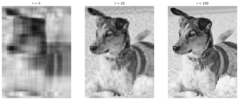
for r in (5, 20, 100):
    # Construct approximate image
    Xapprox = U[:,:r] @ S[0:r,:r] @ VT[:r,:]
    plt.figure(j+1)
    j += 1
    img = plt.imshow(Xapprox)
    img.set_cmap('gray')
    plt.axis('off')
    plt.title('r = ' + str(r))
    plt.show()

原始图片大小：$2000\times 1500=3000000$

当 r = 100 时， 只需要存储 $2000\times 100+100+100\times 1500=350100$，是原始数据的 $\frac{350100}{3000000}=11.67\%$

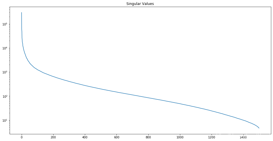
奇异值分布

plt.figure(1)
plt.semilogy(np.diag(S))
plt.title('Singular Values')
plt.show()

semi - log - y : 使用 y 轴的对数坐标作图

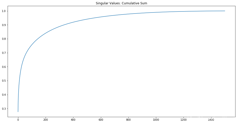
plt.figure(2)
plt.plot(np.cumsum(np.diag(S))/np.sum(np.diag(S)))
plt.title('Singular Values: Cumulative Sum')
plt.show()