吴恩达机器学习课程（第二周）

Linear Regression with Multiple Variables

Enviroment Setup Instruction

Setting Up Programming Assignment Enviroment

Access MATLAB Online and Upload the Programminig Exercise Files

由于电脑已经安装好matlab，所以这节略过。

Multivariate Linear Regression

Multiple Features

这节课中，将介绍一种更为有效的线性回归形式，这种形式适用于多个变量，或者多特征量的情况，叫矩阵乘法。
假如说我有四种特征值，那么：
Notation：
$n$ = number of features
$x^{(i)}$ = input(features) of $i^{th}$training example
${x_j}^{(i)}$ = value of feature j in $i^{th}$ training example
Hypothesis:
$h_{\theta }(x)={\theta }_0+{\theta }_1{x}_1+{\theta }_2{x}_2+{\theta }_3{x}_3+{\theta }_4{x}_4$

那么我们给出多特征值的线性回归预测公式，为了方便，我们定义$x_0=1$
$\begin{array}{l}\mathbf{X}=\left[\begin{array}{l}{x}_0\\ x_1\\ x_2\\ ...\\ x_n\end{array}\right],\theta =\left[\begin{array}{l}{\theta }_0\\ {\theta }_1\\ {\theta }_2\\ ...\\ {\theta }_n\end{array}\right]\\ h_{\theta }(x)={\theta }_0{x}_0+{\theta }_1{x}_1+...+{\theta }_n{x}_n={\theta }^T\mathbf{X}\end{array}$
这就是多元线性回归。

Giadient Descent for Multiple Variables

这节课中，我们将学到如何使用梯度下降法来找的多元线性回归函数的模型参数。
$$\begin{array}{l}\mathrm{H}\mathrm{y}\mathrm{p}\mathrm{o}\mathrm{t}\mathrm{h}\mathrm{e}\mathrm{s}\mathrm{i}\mathrm{s}:h_{\theta }(x)={\theta }_0{x}_0+{\theta }_1{x}_1+...+{\theta }_n{x}_n={\theta }^T\mathbf{X},x_0=1\\ \mathrm{P}\mathrm{a}\mathrm{r}\mathrm{a}\mathrm{m}\mathrm{e}\mathrm{t}\mathrm{e}\mathrm{r}\mathrm{s}:{\theta }_1,{\theta }_2,...,{\theta }_n\\ \mathrm{C}\mathrm{o}\mathrm{s}\mathrm{t}\mathrm{f}\mathrm{u}\mathrm{n}\mathrm{c}\mathrm{t}\mathrm{i}\mathrm{o}\mathrm{n}:\\ \mathrm{J}({\theta }_0,{\theta }_1,...,{\theta }_n)=\frac{1}{2m}\sum _{i=1}^m{\left(h_{\theta }\left(x^{(i)}\right)-y^{(i)}\right)}^2\end{array}$$
G r a d i e n t d e s c e n t : R e p e a t { θ j : = θ j − α ∂ ∂ θ j J ( θ 0 , . . . , θ n ) } ( s i m u l t a n e o u s l y u p d a t e f o r e v e r y j = 0 , . . . , n ) \begin{array}{l} {\rm{Gradient descent:}}\\ {\rm{ \qquad Repeat\{ }}\\ {\rm{ \qquad }}{\theta _j}: = {\theta _j} - \alpha \frac{\partial }{{\partial {\theta _j}}}J({\theta _0},...,{\theta _n})\\ {\rm{\} \qquad \qquad \qquad (simultaneously\quad update\quad for\quad every\quad j = 0,}}...{\rm{,n)}} \end{array} Gradientdescent:Repeat{θj​:=θj​−α∂θj​∂​J(θ0​,...,θn​)}(simultaneouslyupdateforeveryj=0,...,n)​
N e w a l g o r i t h m ( n ≥ 1 ) : R e p e a t { θ j : = θ j − α 1 m ∑ i = 1 m ( h θ ( x ( i ) ) − y ( i ) ) x j ( i ) ( s i m u l r a n e o u s l y u p d a t e θ j f o r j = 0 , . . . , n ) } \begin{array}{l} {\rm{New algorithm(n}} \ge {\rm{1):}}\\ {\rm\qquad\qquad{Repeat\{ }}\\ \qquad\qquad{\theta _j}: = {\theta _j} - \alpha \frac{1}{m}\sum\limits_{i = 1}^m {\left( {{h_\theta }\left( {{x^{(i)}}} \right) - {y^{(i)}}} \right){x_j}^{(i)}} \\ \qquad \qquad\qquad\qquad(simulraneously\quad{\rm\quad{ update }}\quad{\theta _j}\quad for\quad{\rm{ j = 0,}}...{\rm{,n}})\\ {\rm{\} }} \end{array} Newalgorithm(n≥1):Repeat{θj​:=θj​−αm1​i=1∑m​(hθ​(x(i))−y(i))xj​(i)(simulraneouslyupdateθj​forj=0,...,n)}​

Gradient Descent in Practice I-Feature Scaling

在这节课中，我们将学到特征缩放（feature scaling）的方法

feature Scaling

idea:Make sure features are on a similar scale.
当我们把所有特征值都规定到差不多的范围内，收敛的过程就会加快。
E.g.$x_1$=size(0-2000 feet${}_2$)
$x_2$=number of bedroom(1-5)
处理方法：
$\begin{array}{l}{x}_1=\frac{\mathrm{s}\mathrm{i}\mathrm{z}\mathrm{e}(\mathrm{f}\mathrm{e}\mathrm{e}{\mathrm{t}}^2)}{2000}\\ x_2=\frac{\mathrm{n}\mathrm{u}\mathrm{m}\mathrm{b}\mathrm{e}\mathrm{r}\mathrm{o}\mathrm{f}\mathrm{b}\mathrm{e}\mathrm{d}\mathrm{r}\mathrm{o}\mathrm{o}\mathrm{m}\mathrm{s}}{5}\end{array}$
Get every feature into approximately a$-1\le x_i\le 1$range

Mean normalization(均值归一化)

Replace $x_i$with $x_i-{\mu }_i$to make features have approximately zero mean(Do not apply to $x_0=1$)
例如：$\begin{array}{l}{x}_1=\frac{\mathrm{s}\mathrm{i}\mathrm{z}\mathrm{e}-1000}{2000}\\ x_2=\frac{\#\mathrm{b}\mathrm{e}\mathrm{d}\mathrm{r}\mathrm{o}\mathrm{o}\mathrm{m}\mathrm{s}-2}{5}\\ —0.5\le x_1\le 0.5,-0.5\le x_2\le 0.5\end{array}$
$x_1=\frac{x_1-{\mu }_1}{S_1},{\mu }_1=avg,S_1=\max -\min$

Gradient Descent in Practice II-Learning Rate

这节课我们学习的是关于梯度下降算法中的学习率$\alpha$，我们将学到怎么判断梯度下降工作是否正确以及怎么去选择学习率$\alpha$。

Making sure gradient descent is working correctly.

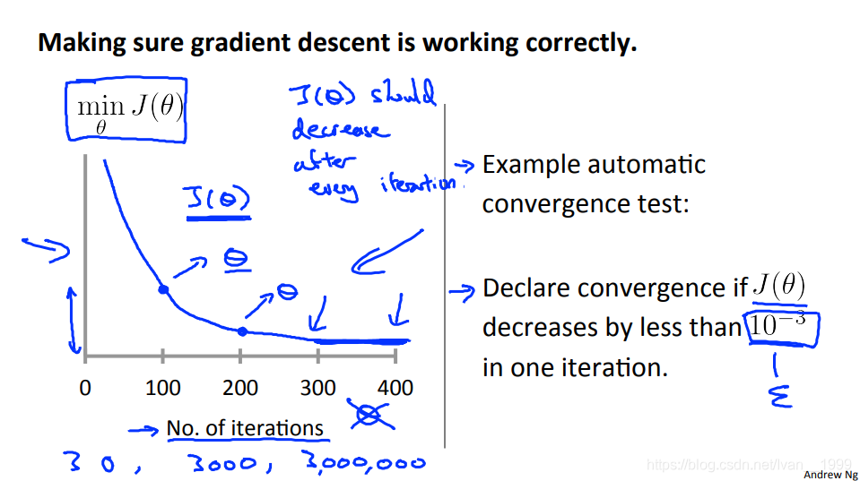
我们直接画出该图，x轴是迭代的次数，y轴是代价函数的值。如果梯度下降正确，那么每一步迭代后，代价函数的值都应该是下降的。
所以当我们的曲线出现不降反升等情况时，我们的学习率就说明设置过高了，如果曲线下降太慢，那说明我们的学习率设置太低了。

Features and Polynomial Regression

这个视频中，将讲到选择特征的方法以及如何得到不同的学习算法。另外会降到多项式回归。
我们在拟合时可以改进一下特征值和假设函数。
我们可以将多个特征值进行结合变成一个，举个例子，我们可以通过$x_1\cdot x_2$变为$x_3$。

多项式回归

当我们的一条直线无法很好的进行拟合时，我们可以改善一下。
我们可以改为为二次，三次，立方根等形式将其变为曲线进行拟合。
还是要记住，均值归一化是非常重要的。

Computing Parameters Analytically

Normal Equation

这个视频中将讲到正规方程（Normal Equation）。
目前我们寻找参数的方法是使用梯度下降法。与之相反的是，正规方程提供了一种求解$\theta$的解析解法，我们可以一次性的求解参数的最优值。
首相，写出我们的代价函数。
$$\theta \in \mathbb{R}{}^{n+1}J({\theta }_0,{\theta }_1,...,{\theta }_m)=\frac{1}{2m}\sum _{i=1}^m{\left(h_{\theta }\left(x^{\left(i\right)}\right)-y^{\left(i\right)}\right)}^2$$
我们只需求每个参数值的偏导，将结果置零，然后求出该参数值，即可得到能够最小化代价函数的参数值。
$$\begin{array}{l}\frac{\partial }{\partial {\theta }_j}J(\theta )=...=0(\mathrm{f}\mathrm{o}\mathrm{r}\mathrm{e}\mathrm{v}\mathrm{e}\mathrm{r}\mathrm{y}\mathrm{j})\\ \mathrm{S}\mathrm{o}\mathrm{l}\mathrm{v}\mathrm{e}\mathrm{f}\mathrm{o}\mathrm{r}{\theta }_0,{\theta }_1,...,{\theta }_n\end{array}$$
下面是我们的计算方法
$$\theta ={\left(X^{T}X\right)}^{-1}{X}^{T}y$$

pinv(X'*X)*X'*y

这个方法不需要进行归一化。
优缺点对比

Gradient Descent	Normal Equation
Need to choose$\alpha$.	No Need to choose$\alpha$.
Needs many iteration.	Don’t need to iterate.
Works well even when feature is large	Need to compute$ \left( {{X^T}X} \right)^{ - 1}$
	Slow if feature is very large

Normal Equation Noninvertibility

这个视频中将讲到正规方程的不可逆性。
我们在线性代数中学到过，有些矩阵是不可逆的，这些不可逆的矩阵叫做奇异矩阵（singular）或退化矩阵（degenerate）。
但如果$ \left( {{X^T}X} \right)^{ - 1}$是不可逆的怎么办？

一般出现这种情况有两种：

• 出现了多余特征值（线性相关）
   比如预测房价时我们有了两个特征值，一个是平方英米，一个是平方米
• 出现了太多特征值（样本数量小于等于特征值数量）
   删除多余特征值，或者进行正则化