


文章来源: 网络
Have you ever wondered how those three little numbers that appear in the UNIX load average(LA) report are calculated?
This online article explains how and how the load average(LA) can be reorganized to do better capacity planning.
1 UNIX Command
...
2 So What Is It
2.1 The man Page
[pax:~] % man "load average"
No manual entry for load average
Oops! There is no man page! The load average metric is am output embedded in other commands so it doesn't get its own man entry. Alright, let's look at the man page for uptime, for example, and see if we can learn more that way.
...
2.2 What the Gurus Have to Say
Let's turn to some UNIX hot-shots for more enlightenment.
Tim O'Reilly and Crew
The book UNIX Power Tools [], tell us on p.726 The CPU:
The load average tries to measure the number of active processes at any time. As a measure of CPU utilization, the load average is simplistic, poorly defined, but far from useless.
That's encouraging! Anyway, it does help to explain what is being measured: the number of active processes. On p.720 39.07 Checking System Load: uptime it continues ...
... High load averages usually mean that the system is being used heavily and the response time is correspondingly slow.
What's high? ... Ideally, you'd like a load average under, say, 3, ... Ultimately, 'high' means high enough so that you don't need uptime to tell you that the system is overloaded.
Hmmm ... where did that number "3" come from? And which of the three averages(1, 5, 15 minutes) are they referring to?
Adrian Cockcroft on Solaris
In Sun Performance and Tuning [] in the section on p.97 entitled: Understanding and Using the Load Average, Adrian Cockcroft states:
The load average is the sum of the run queue length and the number of jobs currently running on the CPUs. In Solaris 2.0 and 2.2 the load average did not include the running jobs but this bug was fixed in Solaris 2.3.
So, even the "big boys" at Sun can get it wrong. Nonetheless, the idea that the load average is associated with the CPU run queue is an important point.
O'Reilly et al. also note some potential gotchas with using load average ...
... different systems will behave differently under the same load average. ... running a single cpu-bound background job ... can bring response to a crawl even though the load avg remains quite low.
As I will demonstrate, this depends on when you look. If the CPU-bound process runs long enough, it will drive the load average up because its always either running or runnable. The obscurities stem from the fact that the load average is not your average kind of average. As we alluded to in the above introduction, it's a time-dependent average. Not only that, but it's a damped time-dependent average. To find out more, let's do some controlled experiments.
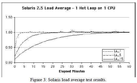
3 Performance Experiments
The experiments described in this section involved running some workloads in background on single-CPU Linux box. There were two phases in the test which has a duration of 1 hour:
- CPU was pegged for 2100 seconds and then the processes were killed.
- CPU was quiescent for the remaining 1500 seconds.
As the authors [] explain about the Linux kernel, because both of our test processes are CPU-bound they will be in a TASK_RUNNING state. This means they are either:
- running i.e., currently executing on the CPU
- runnable i.e., waiting in the run_queue for the CPU
600 * Nr of active tasks - counted in fixed-point numbers
601 */
602 static unsigned long count_active_tasks(void)
603 {
604     struct task_struct *p;
605     unsigned long nr = 0;
606
607     read_lock(&tasklist_lock);
608     for_each_task(p) {
609         if ((p->state == TASK_RUNNING ||
610            (p->state & TASK_UNINTERRUPTIBLE)))
611             nr += FIXED_1;
612     }
613     read_unlock(&tasklist_lock);
614     return nr;
615 }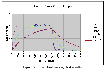
unsigned long avenrun[3];
624
625 static inline void calc_load(unsigned long ticks)
626 {
627     unsigned long active_tasks; /* fixed-point */
628     static int count = LOAD_FREQ;
629
630     count -= ticks;
631     if (count < 0) {
632         count += LOAD_FREQ;
633         active_tasks = count_active_tasks();
634         CALC_LOAD(avenrun[0], EXP_1, active_tasks);
635         CALC_LOAD(avenrun[1], EXP_5, active_tasks);
636         CALC_LOAD(avenrun[2], EXP_15, active_tasks);
637     }
638 }
The countdown is over a LOAD_FREQ of 5 HZ. How often is that?
58 extern unsigned long avenrun[]; /* Load averages */
59
60 #define FSHIFT 11 /* nr of bits of precision */
61 #define FIXED_1 (1<<FSHIFT) /* 1.0 as fixed-point */
62 #define LOAD_FREQ (5*HZ) /* 5 sec intervals */
63 #define EXP_1 1884 /* 1/exp(5sec/1min) as fixed-point */
64 #define EXP_5 2014 /* 1/exp(5sec/5min) */
65 #define EXP_15 2037 /* 1/exp(5sec/15min) */
66
67 #define CALC_LOAD(load,exp,n) \
68 load *= exp; \
69 load += n*(FIXED_1-exp); \
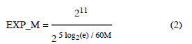
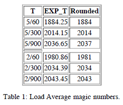
70 load >>= FSHIFT;A noteable curiosity is the appearance of those magic numbers: 1884, 2014, 2037. What do they mean? If we look at the preamble to the code we learn,
/*
* These are the constant used to fake the fixed-point load-average
50 * counting. Some notes:
51 * - 11 bit fractions expand to 22 bits by the multiplies: this gives
52 * a load-average precision of 10 bits integer + 11 bits fractional
53 * - if you want to count load-averages more often, you need more
54 * precision, or rounding will get you. With 2-second counting freq,
55 * the EXP_n values would be 1981, 2034 and 2043 if still using only
56 * 11 bit fractions.
57 */
These magic numbers are a result of using a fixed-point ( rather than a floating-pointer ) representation.
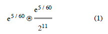
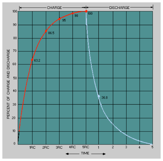
One question still remains, however. Where do the ratios like exp(5/60) come from?
4.2 Magic Revealed
Taking the 1-minute average as the example, CALC_LOAD is identical to the mathematical expression:


Conversely, when n = 2 as it was in our experiments, the load average is dominated by the second term such that:

5 Summary
So, what have we learned? Those three innocious looking numbers in the LA triplet have a surprising amount of depth behind them.
The triplet is intended to provide you with some kind of information about how much work has been done on the system in the recent past (1 minute), the past(5 minute) and the distant past(15 minutes).
As you will now appreciate, there are some issues:
1. The "load" is not the utilization but the total queue length.
2. They are point samples of three different time series.
3. They are exponentially - damped moving averages.
4. They are in the wrong order to represent trend information.
These inherited limitations are significant if you try to use them for capacity planning purpose. I'll have more to say about all this in the next online column Load Average Part II : Not Your Average Average.


 8710
8710

 被折叠的 条评论
为什么被折叠?
被折叠的 条评论
为什么被折叠?
 到【灌水乐园】发言


