第3章 Python 数字图像处理(DIP) - 灰度变换与空间滤波15 - 锐化高通滤波器 -拉普拉斯核（二阶导数）

锐化（高通）空间滤波器

• 平滑通过称为低通滤波
• 类似于积分运算
• 锐化通常称为高通滤波
• 微分运算
• 高过（负责细节的）高频，衰减或抑制低频

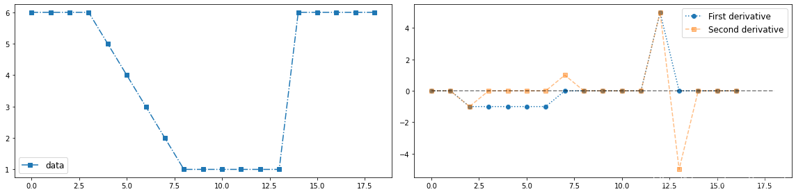
基础 - 一阶导数和二阶导数的锐化滤波器

数字函数的导数是用差分来定义的。定义这些差分的方法有多种

一阶导数的任何定义都要满足如下要求：

1. 恒定灰度区域的一阶导数必须为0
2. 灰度台阶或斜坡开始处的一阶导数必须非零。
3. 灰度斜坡上的一阶导数必须非零。

二阶导数的任何定义都要满足如下要求：

1. 恒定灰度区域的二阶导数必须为零。
2. 灰度台阶或斜坡的开始处和结束处的地阶导数必须非零。
3. 灰度斜坡上的二阶导数必须为零。

一维函数$f(x)$的一阶导数的一个基本定义是差分：
$$\frac{\partial f}{\partial x}=f(x+1)-f(x)\text{\hspace{1em}(3.48)}$$

二阶导数定义为差分：
$$\frac{{\partial }^{2}f}{\partial x^2}=f(x+1)+f(x-1)-2f(x)\text{\hspace{1em}(3.49)}$$

def first_derivative(y):
    y_1 = np.zeros(len(y)-1)
    for i in range(1, len(y)):
        if i + 1 < len(y):
            y_1[i] = y[i+1] - y[i]
    return y_1

def second_derivative(y):
    y_2 = np.zeros(len(y)-1)
    for i in range(1, len(y)):
        if i + 1 < len(y):
            y_2[i] = y[i+1] + y[i-1] - 2*y[i]
    return y_2

#一维数字一阶与二阶导数
y = np.arange(1, 7)
y = y[::-1]
y = np.pad(y, (3, 5), mode='constant', constant_values=(6, 1))
y = np.pad(y, (0, 5), mode='constant', constant_values=(0, 6))
x = np.arange(len(y))

fig = plt.figure(figsize=(16, 4))
ax_1 = fig.add_subplot(1, 2, 1)
ax_1.plot(x, y, '-.s', label="data")
ax_1.legend(loc='best', fontsize=12)

y_1 = first_derivative(y)
y_2 = second_derivative(y)

ax_2 = fig.add_subplot(1, 2, 2)
ax_2.plot(y_1[1:], ':o', label='First derivative')
ax_2.plot(y_2[1:], '--s', alpha=0.5, label='Second derivative')
ax_2.plot(np.zeros(19), '--k', alpha=0.5)
ax_2.legend(loc='best', fontsize=12)
plt.tight_layout()
plt.show()

二阶导数锐化图像–拉普拉斯

我们感兴趣的是各向同性核，这种核的响应与图像中灰度不连续的方向无关。最简单的各向同性导数算子（核）是拉普拉斯， 它定义为：
$${\nabla }^{2}f=\frac{{\partial }^{2}f}{\partial x^2}+\frac{{\partial }^{2}f}{\partial y^2}\text{\hspace{1em}(3.50)}$$

我们把这个片子以离散形式表达:
$$\frac{{\partial }^{2}f}{\partial x^2}=f(x+1,y)+f(x-1,y)-2f(x,y)\text{\hspace{1em}(3.51)}$$
$$\frac{{\partial }^{2}f}{\partial y^2}=f(x,y+1)+f(x,y-1)-2f(x,y)\text{\hspace{1em}(3.52)}$$

两个变量的离散拉普拉斯是
$${\nabla }^{2}f(x,y)=f(x+1,y)+f(x-1,y)+f(x,y+1)+f(x,y-1)-4f(x,y)\text{\hspace{1em}(3.53)}$$

写成矩阵的形式就得到拉普拉斯核：
$$\left[\begin{array}{ccc}0& 1(f(x,y-1)的权值)& 0\\ 1(f(x-1,y)的权值)& -4(f(x,y)的权值)& 1(f(x+1,y)的权值)\\ 0& 1(f(x,y+1)的权值)& 0\end{array}\right]$$

图像的锐化的滤波原理也类似于描述的低通滤波，只不过使用不同的系数
后面两个是含对角项的扩展公式的核：

$\left[\begin{array}{ccc}0& 1& 0\\ 1& -4& 1\\ 0& 1& 0\end{array}\right]\left[\begin{array}{ccc}1& 1& 1\\ 1& -8& 1\\ 1& 1& 1\end{array}\right]$

这两个是二阶导数定义得到的：

$\left[\begin{array}{ccc}0& -1& 0\\ -1& 4& -1\\ 0& -1& 0\end{array}\right]\left[\begin{array}{ccc}-1& -1& -1\\ -1& 8& -1\\ -1& -1& -1\end{array}\right]$

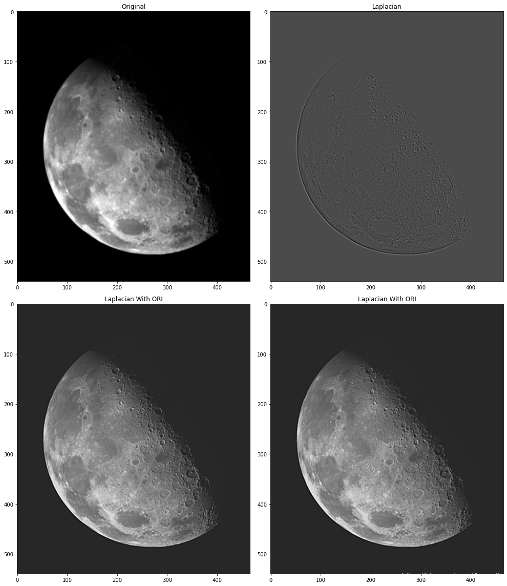
拉普拉斯是导数算子，因此会突出图像中的急剧灰度过渡，并且不会强调缓慢变化的灰度区域。这往往会产生具有灰色边缘线和其他不连续性的图像，它们都叠加在暗色无特征背景上。将拉普拉斯图像与原图相加，就可以“恢复”背景特征，同时保留拉普拉斯的锐化效果。 上面两个核得到的图像需要用原图减去得到的图，下面两个核得到的图像需要用原图加下得到的图，以实现锐化。

$$g(x,y)=f(x,y)+c[{\nabla }^{2}f(x,y)]\text{\hspace{1em}(3.54)}$$
使用上面的前两个核，则$c=-1$，后面的两个二阶导数定义的核则$c=1$
两组核刚好相差一个负号

观察平滑与锐化核可发现，平滑核的系数之和为1，锐化核的系数之和为0。用锐化核处理图像时，有会出现负值，需要进行额外处理才能得到合适的视觉结果。

# Laplacian filter 不同的核，拉普拉斯锐化
img = cv2.imread('DIP_Figures/DIP3E_Original_Images_CH03/Fig0338(a)(blurry_moon).tif', 0)
img = normalize(img)

kernel_laplacian_a = np.array([
                    [0,1,0],
                    [1,-4,1],
                    [0,1,0]])
# 下面这个核虽然可以锐化，但是效果没有上面这个好
# kernel_laplacian_d = np.array([[
#                     [-1, -1, -1],
#                     [-1, 8, -1],
#                     [-1, -1, -1]
#                                 ]])
laplacian_img_a = filter_2d(img, kernel_laplacian_a, mode='constant')
laplacian_img_b = filter_2d(img, -kernel_laplacian_a, mode='constant')

plt.figure(figsize=(14, 16))
plt.subplot(2, 2, 1), plt.imshow(img, cmap='gray', vmin=0, vmax=1), plt.title('Original')
plt.subplot(2, 2, 2), plt.imshow(laplacian_img_a, cmap='gray', vmax=1), plt.title('Laplacian')

laplacian_img_ori = normalize(img - laplacian_img_a)
plt.subplot(2, 2, 3), plt.imshow(laplacian_img_ori, cmap='gray', vmax=1), plt.title('Laplacian With ORI')

laplacian_imgori = normalize(img + laplacian_img_b)
plt.subplot(2, 2, 4), plt.imshow(laplacian_imgori, cmap='gray', vmax=1), plt.title('Laplacian With ORI')

plt.tight_layout()
plt.show()