第5章 Python 数字图像处理(DIP) - 图像复原与重建1 - 高斯噪声

本章主要讲图像复原与重建，首先是了解一下各种噪声的特点与模型，还有形成的方法。一些重点的噪声，如高斯噪声，均匀噪声，伽马噪声，指数噪声，还有椒盐噪声等。
本章主要的噪声研究方法主要是加性噪声。

import sys
import numpy as np
import cv2
import matplotlib 
import matplotlib.pyplot as plt
import PIL
from PIL import Image

print(f"Python version: {sys.version}")
print(f"Numpy version: {np.__version__}")
print(f"Opencv version: {cv2.__version__}")
print(f"Matplotlib version: {matplotlib.__version__}")
print(f"Pillow version: {PIL.__version__}")

Python version: 3.7.6 (default, Jan  8 2020, 20:23:39) [MSC v.1916 64 bit (AMD64)]
Numpy version: 1.18.1
Opencv version: 4.2.0
Matplotlib version: 3.1.3
Pillow version: 7.0.0

def normalize(mask):
    return (mask - mask.min()) / (mask.max() - mask.min())

图像退化/复原处理的一个模型

• 退化
  把图像退化建模为一个算子$\mathcal{H}$，算子与一个加性噪声项共同对输入图像$f(x,y)$进行运算，生成一幅退化的图像$g(x,y)$。

• 复原
  已知退化图像$g(x,y)$、关于$\mathcal{H}$和加性噪声项$\eta (x,y)$，要复原的目的是得到原图的一个估计$\hat{f}(x,y)$，并使得与$f(x,y)$尽可能接近。

• 退化模型
  $$f(x,y)\Rightarrow 退化函数\mathcal{H}\Rightarrow \oplus 噪声\eta (x,y)\Rightarrow g(x,y)$$

• 复原模型
  $$g(x,y)\Rightarrow 复原滤波器\Rightarrow \hat{f}(x,y)$$

若$\mathcal{H}$是一个线性位置不变片子，则空间域中的退化图像为

$$g(x,y)=(h\star f)(x,y)+\eta (x,y)\text{\hspace{1em}(5.1)}$$
频率域的等效公式为
$$G(u,v)=H(u,v)F(u,v)+N(u,v)\text{\hspace{1em}(5.2)}$$

噪声模型

噪声的空间和频率特性

当噪声的傅里叶谱是常量时，噪声通常称为白噪声

一些重要的噪声概率密度函数（PDF）

高斯噪声

高斯随机变量的PDF如下
$$P(z)=\frac{1}{\sqrt{2\pi \sigma }}{e}^{-(z-\bar{z}{)}^2/2{\sigma }^2},-\infty <z<\infty \text{\hspace{1em}(5.3)}$$

式中，$z$表示灰度，$\bar{z}$是$z$的均（平均）值，$\sigma$是$z$的标准差。$z$值在区间$\bar{z}\pm \sigma$内的概率约为0.68，$z$值在区间$\bar{z}\pm 2\sigma$内的概率约为0.95。

def gauss_pdf(z):
    
    mean = np.mean(z)
    sigma = np.std(z)
    gauss = (1 /(np.sqrt(2*np.pi*sigma))) * np.exp(-((z - mean)**2)/(2*sigma))
    
    return gauss

更正下面代码，如果之前已经复制的，也请更正

def add_gaussian_noise(img, mu=0, sigma=0.1):
    """
    add gaussian noise for image
    param:  img:       input image, dtype=uint8
    param:  mean:      noise mean
    param:  sigma:     noise sigma
    return: image_out: image with gaussian noise
    """
    # image = np.array(img/255, dtype=float) # 这是有错误的，将得不到正确的结果，修改如下
    image = np.array(img, dtype=float)
    noise = np.random.normal(mu, sigma, image.shape)

    # 这是另外一种采样法，但不是很正确
#     x = np.linspace(-(mu + 10 * sigma), (mu + 10 * sigma), 500)
#     gauss = 1/(np.sqrt(2 * np.pi) * sigma) * np.exp(-(x - mu)**2 / (2 * sigma**2))
#     gauss = gauss / gauss.max()
#     noise = np.random.choice(gauss, size=image.shape)
    
    image_out = image + noise
    image_out = np.uint8(normalize(image_out)*255)
    
    return image_out    

# 高斯PDF
mean = 0 
sigma = 20
image = np.zeros([512, 512])
noise = np.random.normal(mean, sigma, image.shape)
z_ = np.mean(noise)
sigma = np.std(noise)
print(f"z_ -> {z_}, sigma^2 -> {sigma}")

# noise_max = max(abs(noise.min()), noise.max())
# # noise = noise_max - noise
# noise = noise / noise_max

z_ = np.mean(noise)
sigma = np.std(noise)
print(f"z_ -> {z_}, sigma^2 -> {sigma}")
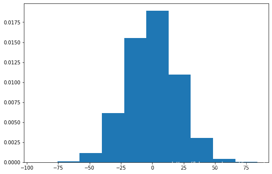
plt.figure(figsize=(9, 6))
hist = plt.hist(noise.flatten(), density=True)
plt.show()

z_ -> -0.017029652654878595, sigma^2 -> 20.04642811124816
z_ -> -0.017029652654878595, sigma^2 -> 20.04642811124816

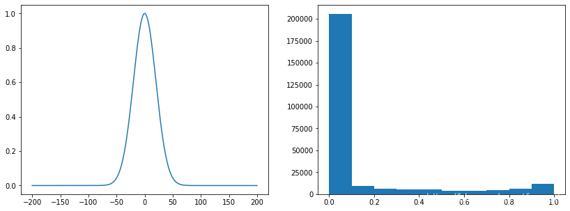
# 采样
mu = 0
sigma = 20
x = np.linspace(-(mu + 10 * sigma), (mu + 10 * sigma), 500)
gauss = 1/(np.sqrt(2 * np.pi) * sigma) * np.exp(-(x - mu)**2 / (2 * sigma**2))
gauss = gauss / gauss.max()
choice = np.random.choice(gauss, size=image.shape)

plt.figure(figsize=(14, 5))
plt.subplot(1,2,1), plt.plot(x, gauss)
plt.subplot(1,2,2), plt.hist(choice.flatten())
plt.show()

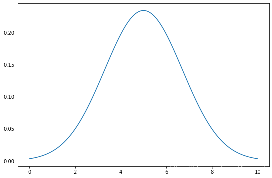
# 高斯PDF
z = np.linspace(0, 10, 500)

z_ = np.mean(z)
sigma = np.std(z)

print(f"z_ -> {z_}, sigma^2 -> {sigma}")
gauss = gauss_pdf(z)

plt.figure(figsize=(9, 6))
plt.plot(z, gauss)
plt.show()

z_ -> 5.0, sigma^2 -> 2.8925306337070777

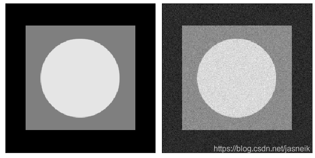
# 高斯加性噪声
img_ori = cv2.imread("DIP_Figures/DIP3E_Original_Images_CH05/Fig0503 (original_pattern).tif", 0)
# img_ori = np.ones([256, 256]) * 128
img_gauss = add_gaussian_noise(img_ori, mu=0, sigma=10) # Fix 2021-12-16, image show below donot fixed, so the result might be not the same

plt.figure(figsize=(9, 6))
plt.subplot(121), plt.imshow(img_ori, 'gray', vmin=0, vmax=255), plt.xticks([]), plt.yticks([])
plt.subplot(122), plt.imshow(img_gauss, 'gray'), plt.xticks([]), plt.yticks([])

plt.tight_layout()
plt.show()

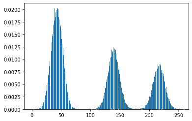
hist, bins = np.histogram(img_gauss.flatten(), bins=255, range=[0, 255], density=True)
bar = plt.bar(bins[:-1], hist[:])