Tensorflow基本语法和实现神经网络

1. 基本语法

        一般我们在用tensorflow编程时，会分为以下几个步骤：

• 创建Tensors(变量)
• 编写Tensors间的操作符
• 初始化Tensors
• 创建一个Session
• 运行Session

       示例如下：

y_hat = tf.constant(36, name='y_hat')            # 定义一个常量y_hat,赋值为36
y = tf.constant(39, name='y')                    # 定义一个常量，赋值为39

loss = tf.Variable((y - y_hat)**2, name='loss')  # 创建一个变量

init = tf.global_variables_initializer()         # 当执行(session.run(init))时，
                                                 # 变量loss会被初始化并且做好了计算的准备
with tf.Session() as session:                    # 创建一个Session用于print输出
    session.run(init)                            # 初始化变量
    print(session.run(loss))                     # 运行Session并输出loss

        有时候，我们需要先定义一个变量，然后在运行的时候才进行赋值，这就是tensorflow的placeholder对象了。基本用法就是先创建一个placeholder对象，然后在调用的时候通过feed_dict把值传过去，示例如下：

def sigmoid(z):
   
    # 创建一个placeholder对象x
    x = tf.placeholder(tf.float32, name = "x")

    # 利用tf的sigmoid()函数计算sigmod
    sigmoid = tf.sigmoid(x)

    # 创建一个session并运行
    # 通过feed_dict把z的值传给x 
    with tf.Session() as sess:
        # 运行session然后染回"result"
        result = sess.run(sigmoid, feed_dict = {x : z})
    
    return result

2. 实现神经网络

2.1 数据集准备

加载数据：

# Loading the dataset
X_train_orig, Y_train_orig, X_test_orig, Y_test_orig, classes = load_dataset()

数据处理：把数据处理成可以直接用在模型上的格式，代码如下：

# 把训练集和测试集的图像展开
X_train_flatten = X_train_orig.reshape(X_train_orig.shape[0], -1).T
X_test_flatten = X_test_orig.reshape(X_test_orig.shape[0], -1).T
# 归一化
X_train = X_train_flatten/255.
X_test = X_test_flatten/255.
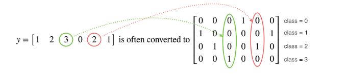
# 把训练集和测试集的标签转换成一个hot矩阵
Y_train = convert_to_one_hot(Y_train_orig, 6)
Y_test = convert_to_one_hot(Y_test_orig, 6)

        这里的one hot编码，如下图所示：

2.2 定义placeholder

       为了在运行session时把训练数据传过去，需要定义placeholder，代码如下：

def create_placeholders(n_x, n_y):
    """
    Creates the placeholders for the tensorflow session.
    
    Arguments:
    n_x -- scalar, size of an image vector (num_px * num_px = 64 * 64 * 3 = 12288)
    n_y -- scalar, number of classes (from 0 to 5, so -> 6)
    
    Returns:
    X -- placeholder for the data input, of shape [n_x, None] and dtype "float"
    Y -- placeholder for the input labels, of shape [n_y, None] and dtype "float"
    
    Tips:
    - You will use None because it let's us be flexible on the number of examples you will for the placeholders.
      In fact, the number of examples during test/train is different.
    """

    ### START CODE HERE ### (approx. 2 lines)
    X = tf.placeholder(tf.float32, shape = [n_x, None], name = "X")
    Y = tf.placeholder(tf.float32, shape = [n_y, None], name = "Y")
    ### END CODE HERE ###
    
    return X, Y

2.3 参数初始化

代码如下：

def initialize_parameters():
    """
    Initializes parameters to build a neural network with tensorflow. The shapes are:
                        W1 : [25, 12288]
                        b1 : [25, 1]
                        W2 : [12, 25]
                        b2 : [12, 1]
                        W3 : [6, 12]
                        b3 : [6, 1]
    
    Returns:
    parameters -- a dictionary of tensors containing W1, b1, W2, b2, W3, b3
    """
    
    tf.set_random_seed(1)                   # so that your "random" numbers match ours
        
    ### START CODE HERE ### (approx. 6 lines of code)
    W1 = tf.get_variable("W1", shape = [25, 12288], initializer = tf.contrib.layers.xavier_initializer(seed = 1))
    b1 = tf.get_variable("b1", shape = [25, 1], initializer = tf.zeros_initializer())
    W2 = tf.get_variable("W2", shape = [12, 25], initializer = tf.contrib.layers.xavier_initializer(seed = 1))
    b2 = tf.get_variable("b2", shape = [12, 1], initializer = tf.zeros_initializer())
    W3 = tf.get_variable("W3", shape = [6, 12], initializer = tf.contrib.layers.xavier_initializer(seed = 1))
    b3 = tf.get_variable("b3", shape = [6, 1], initializer = tf.zeros_initializer())
    ### END CODE HERE ###

    parameters = {"W1": W1,
                  "b1": b1,
                  "W2": W2,
                  "b2": b2,
                  "W3": W3,
                  "b3": b3}
    
    return parameters

2.4 前向传播

代码如下：

# GRADED FUNCTION: forward_propagation

def forward_propagation(X, parameters):
    """
    Implements the forward propagation for the model: LINEAR -> RELU -> LINEAR -> RELU -> LINEAR -> SOFTMAX
    
    Arguments:
    X -- input dataset placeholder, of shape (input size, number of examples)
    parameters -- python dictionary containing your parameters "W1", "b1", "W2", "b2", "W3", "b3"
                  the shapes are given in initialize_parameters

    Returns:
    Z3 -- the output of the last LINEAR unit
    """
    
    # Retrieve the parameters from the dictionary "parameters" 
    W1 = parameters['W1']
    b1 = parameters['b1']
    W2 = parameters['W2']
    b2 = parameters['b2']
    W3 = parameters['W3']
    b3 = parameters['b3']
    
    ### START CODE HERE ### (approx. 5 lines)              # Numpy Equivalents:
    Z1 = tf.add(tf.matmul(W1, X), b1)                                             # Z1 = np.dot(W1, X) + b1
    A1 = tf.nn.relu(Z1)                                              # A1 = relu(Z1)
    Z2 = tf.add(tf.matmul(W2, A1), b2)                                              # Z2 = np.dot(W2, a1) + b2
    A2 = tf.nn.relu(Z2)                                              # A2 = relu(Z2)
    Z3 = tf.add(tf.matmul(W3, A2), b3)                                              # Z3 = np.dot(W3,Z2) + b3
    ### END CODE HERE ###
    
    return Z3

2.5 计算代价函数

def compute_cost(Z3, Y):
    """
    Computes the cost
    
    Arguments:
    Z3 -- output of forward propagation (output of the last LINEAR unit), of shape (6, number of examples)
    Y -- "true" labels vector placeholder, same shape as Z3
    
    Returns:
    cost - Tensor of the cost function
    """
    
    # to fit the tensorflow requirement for tf.nn.softmax_cross_entropy_with_logits(...,...)
    logits = tf.transpose(Z3)
    labels = tf.transpose(Y)
    
    ### START CODE HERE ### (1 line of code)
    cost = tf.reduce_mean(tf.nn.softmax_cross_entropy_with_logits(logits = logits, labels = labels))
    ### END CODE HERE ###
    
    return cost

2.6 后向传播和参数更新

       tensorflow封装了这个过程，所有的反向传播和参数更新只需要一行代码就可以完成。当你计算完代价函数之后，只需要创建一个“optimizer”对象。 在运行tf.session时，必须调用这个“optimizer”对象和成本函数。“optimizer”对象被调用时，它将根据所选择的梯度下降方法和learning rate对给定的代价函数进行优化。代码如下：

optimizer = tf.train.GradientDescentOptimizer(learning_rate = learning_rate).minimize(cost) # 创建optimizer对象
_ , c = sess.run([optimizer, cost], feed_dict={X: minibatch_X, Y: minibatch_Y}) # 执行反向传播及参数更新

       一般，"_"表示作为“一次性”变量来存储我们以后不需要使用的值。

2.7 定义神经网络模型

def model(X_train, Y_train, X_test, Y_test, learning_rate = 0.0001,
          num_epochs = 1500, minibatch_size = 32, print_cost = True):
    """
    实现一个3层tensorflow神经网络: LINEAR->RELU->LINEAR->RELU->LINEAR->SOFTMAX.
    
    输入参数:
    X_train -- 训练集, (输入特征数 = 12288, 样例数 = 1080)
    Y_train -- 训练集, (输出维度 = 6, 样例数 = 1080)
    X_test -- 测试集, (输入特征数 = 12288, 样例数 = 120)
    Y_test -- 测试集, (输入特征数 = 12288, 样例数 = 120)
    learning_rate -- 参数更新的learning rate
    num_epochs -- 迭代次数
    minibatch_size -- minibatch大小
    print_cost -- 是否每迭代100输出代价
    
    返回参数:
    parameters -- 学习到的模型参数，用于预测新的数据集.
    """
    
    ops.reset_default_graph()   # to be able to rerun the model without overwriting tf variables
    tf.set_random_seed(1)       # to keep consistent results
    seed = 3                    # to keep consistent results
    (n_x, m) = X_train.shape    # (n_x: input size, m : number of examples in the train set)
    n_y = Y_train.shape[0]      # n_y : output size
    costs = []                  # To keep track of the cost
    
    # 创建 Placeholders 
    X, Y = create_placeholders(n_x, n_y)
    

    # 初始化参数
    parameters = initialize_parameters()
    
    # 前向传播: 用tensorflow graph建立前向传播
    Z3 = forward_propagation(X, parameters)
    
    # 计算代价
    cost = compute_cost(Z3, Y)
    
    # 后向传播: 定义tensorflow optimizer对象，这里使用AdamOptimizer.
    optimizer = tf.train.AdamOptimizer(learning_rate = learning_rate).minimize(cost)
    
    # 初始化所有的参数
    init = tf.global_variables_initializer()

    # 启动session来计算tensorflow graph
    with tf.Session() as sess:
        
        # Run the initialization
        sess.run(init)
        
        # 循环迭代
        for epoch in range(num_epochs):

            epoch_cost = 0.                       # 定义每一大次迭代的代价
            num_minibatches = int(m / minibatch_size) # 训练集minibatch的数量
            seed = seed + 1
            minibatches = random_mini_batches(X_train, Y_train, minibatch_size, seed)

            for minibatch in minibatches:

                # 选择一个minibatch
                (minibatch_X, minibatch_Y) = minibatch
                
                # IMPORTANT: The line that runs the graph on a minibatch.
                # Run the session to execute the "optimizer" and the "cost", the feedict should contain a minibatch for (X,Y).
                _ , minibatch_cost = sess.run([optimizer, cost], feed_dict = {X : minibatch_X, Y: minibatch_Y})
                
                epoch_cost += minibatch_cost / num_minibatches

            # Print the cost every epoch
            if print_cost == True and epoch % 100 == 0:
                print ("Cost after epoch %i: %f" % (epoch, epoch_cost))
            if print_cost == True and epoch % 5 == 0:
                costs.append(epoch_cost)
                
        # plot the cost
        plt.plot(np.squeeze(costs))
        plt.ylabel('cost')
        plt.xlabel('iterations (per tens)')
        plt.title("Learning rate =" + str(learning_rate))
        plt.show()

        # lets save the parameters in a variable
        parameters = sess.run(parameters)
        print ("Parameters have been trained!")

        # Calculate the correct predictions
        correct_prediction = tf.equal(tf.argmax(Z3), tf.argmax(Y))

        # Calculate accuracy on the test set
        accuracy = tf.reduce_mean(tf.cast(correct_prediction, "float"))

        print ("Train Accuracy:", accuracy.eval({X: X_train, Y: Y_train}))
        print ("Test Accuracy:", accuracy.eval({X: X_test, Y: Y_test}))
        
        return parameters

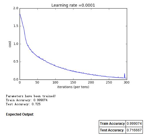
2.8 模型调用

parameters = model(X_train, Y_train, X_test, Y_test)

3. 实验结果