


 本文从线性可分和支持向量机(SVM)的概念出发,介绍了SVM的基本原理及其在人脸识别中的应用。通过实例展示了如何使用Python的sklearn库进行SVM模型训练和测试。
本文章内容来自麦子学院课程-机器学习,特此申明。注:更多资源及软件请W信关注“学娱汇聚门”
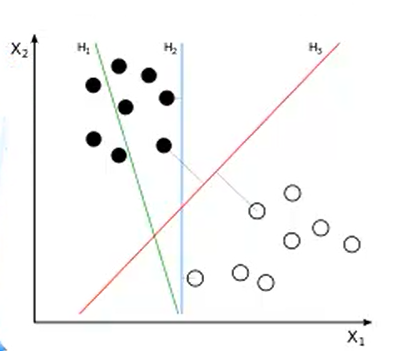
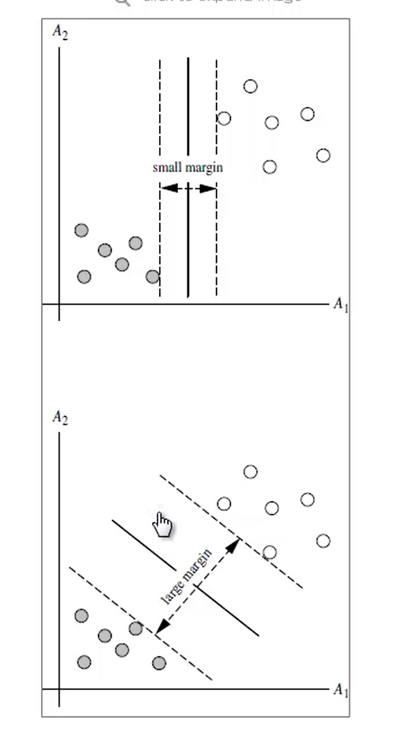
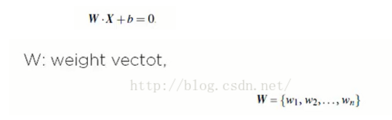
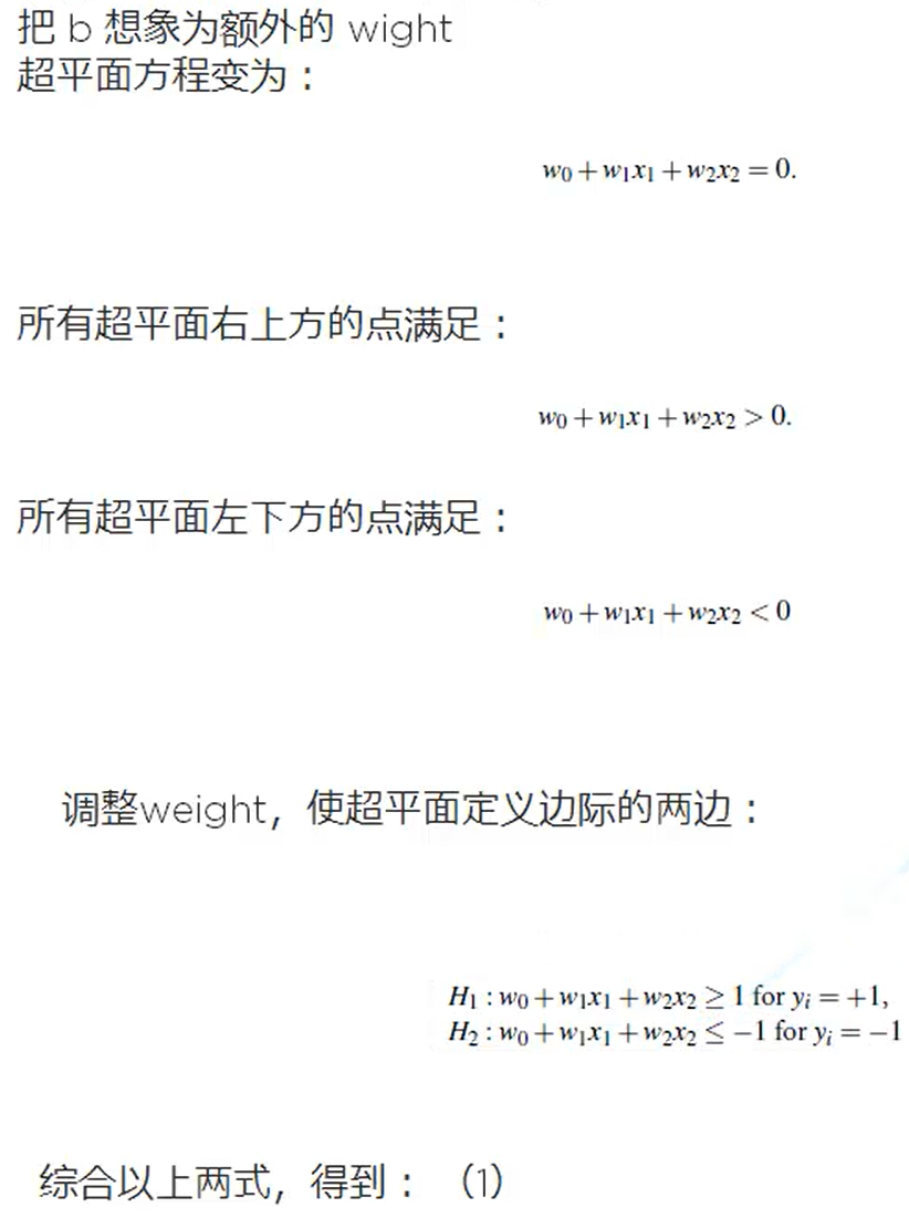
Part One:线性可分的SVM
1. SVM 背景
3.1 例子:
例题1:

from sklearn import svm

X = [[2, 0], [1, 1], [2,3]]
y = [0, 0, 1]
clf = svm.SVC(kernel = 'linear')
clf.fit(X, y)

print clf

# get support vectors
print clf.support_vectors_

# get indices of support vectors
print clf.support_

# get number of support vectors for each class
print clf.n_support_
例题2:
print(__doc__)

import numpy as np
import pylab as pl
from sklearn import svm

# we create 40 separable points
np.random.seed(0)
X = np.r_[np.random.randn(20, 2) - [2, 2], np.random.randn(20, 2) + [2, 2]]
Y = [0] * 20 + [1] * 20

# fit the model
clf = svm.SVC(kernel='linear')
clf.fit(X, Y)

# get the separating hyperplane
w = clf.coef_[0]

a = -w[0] / w[1]
xx = np.linspace(-5, 5)
yy = a * xx - (clf.intercept_[0]) / w[1]

# plot the parallels to the separating hyperplane that pass through the
# support vectors
b = clf.support_vectors_[0]
yy_down = a * xx + (b[1] - a * b[0])
b = clf.support_vectors_[-1]
yy_up = a * xx + (b[1] - a * b[0])


print("w: ", w)
print("a: ", a)
# print " xx: ", xx
# print " yy: ", yy
print("support_vectors_: ", clf.support_vectors_)
print("clf.coef_: ", clf.coef_)

# In scikit-learn coef_ attribute holds the vectors of the separating hyperplanes for linear models. It has shape (n_classes, n_features) if n_classes > 1 (multi-class one-vs-all) and (1, n_features) for binary classification.
#
# In this toy binary classification example, n_features == 2, hence w = coef_[0] is the vector orthogonal to the hyperplane (the hyperplane is fully defined by it + the intercept).
#
# To plot this hyperplane in the 2D case (any hyperplane of a 2D plane is a 1D line), we want to find a f as in y = f(x) = a.x + b. In this case a is the slope of the line and can be computed by a = -w[0] / w[1].


# plot the line, the points, and the nearest vectors to the plane
pl.plot(xx, yy, 'k-')
pl.plot(xx, yy_down, 'k--')
pl.plot(xx, yy_up, 'k--')

pl.scatter(clf.support_vectors_[:, 0], clf.support_vectors_[:, 1],
           s=80, facecolors='none')
pl.scatter(X[:, 0], X[:, 1], c=Y, cmap=pl.cm.Paired)

pl.axis('tight')
pl.show()
运行结果图如下:

结果数据:
w: [ 0.90230696 0.64821811]
a: -1.39198047626
support_vectors_: [[-1.02126202 0.2408932 ]
[-0.46722079 -0.53064123]
[ 0.95144703 0.57998206]]
clf.coef_: [[ 0.90230696 0.64821811]]
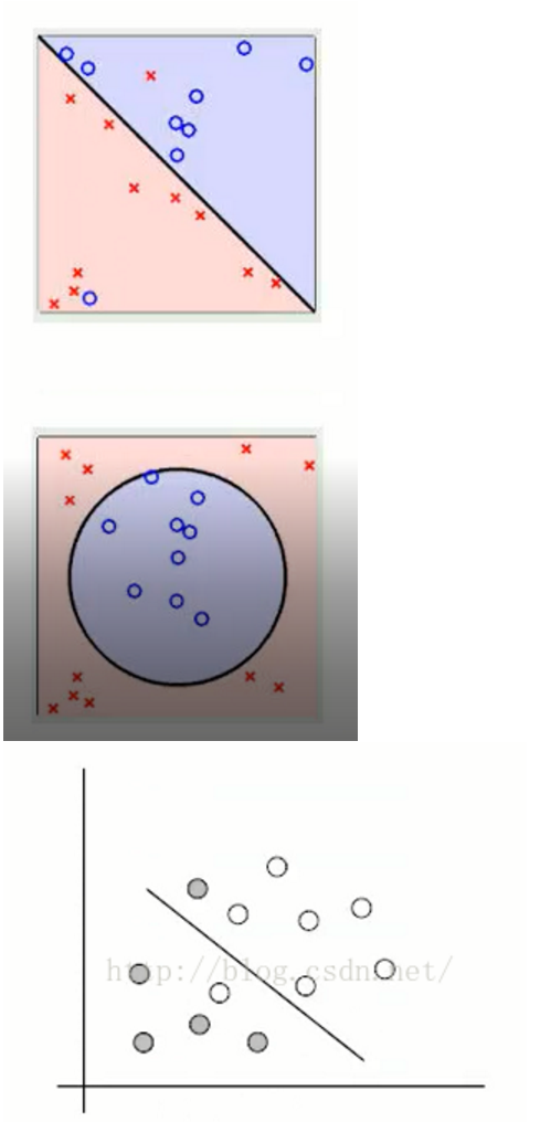
Part Two:线性不可分的SVM
根据前面的内容我们测试的是线性可分的SVM,以下为线性不可分的SVM实现原理及例程:
1. SVM算法特性:
1.1 训练好的模型的算法复杂度是由支持向量的个数决定的,而不是由数据的维度决定的。所以SVM不太容易产生overfitting
1.2 SVM训练出来的模型完全依赖于支持向量(Support Vectors), 即使训练集里面所有非支持向量的点都被去除,重复训练过程,结果仍然会得到完全一样的模型。
1.3 一个SVM如果训练得出的支持向量个数比较小,SVM训练出的模型比较容易被泛化。


例子:以下为人脸识别的算法实现
from __future__ import print_function

from time import time      #有此步骤要计时,看花了多少时间
import logging             #打印进展信息
import matplotlib.pyplot as plt       #最后需要把我们识别出来的人脸,用图来绘制出来
#以下为sklearn包
from sklearn.cross_validation import train_test_split
from sklearn.datasets import fetch_lfw_people
from sklearn.grid_search import GridSearchCV
from sklearn.metrics import classification_report
from sklearn.metrics import confusion_matrix
from sklearn.decomposition import RandomizedPCA
from sklearn.svm import SVC
# 显示进度和错误信息,basicConfig:把程序中的进展的参数打印出来
logging.basicConfig(level=logging.INFO, format='%(asctime)s %(message)s')


###############################################################################
#fetch_lfw_people用于下载名人的人脸库的,下载的数据集地址:http://vis-www.cs.umass.edu/lfw/index.html
lfw_people = fetch_lfw_people(min_faces_per_person=70, resize=0.4)

# 转换为数组
n_samples, h, w = lfw_people.images.shape     #n_samples=1288为多少个实例,h=50,w=37,即1288*50*37

# 对于机器学习,我们直接使用2个数据(由于该模型忽略了相对像素位置信息)  X每行是实例,每列为特征值。
X = lfw_people.data
n_features = X.shape[1]       #每个人可以获得多少个特征值 n_features=1850

# 预测的标签是该人的身份
y = lfw_people.target                     #每个实例对应的人名,即标记,1288维
target_names = lfw_people.target_names    #返回所有人的名字,7*1维tuple
n_classes = target_names.shape[0]         #看有多少个人?即多少类?n_classes=7

print("Total dataset size:")
print("n_samples: %d" % n_samples)
print("n_features: %d" % n_features)
print("n_classes: %d" % n_classes)


###############################################################################
# 分为训练集和使用分层k折的测试集

# 分为训练集和测试集,X_train为训练集的特征向量, y_train为训练集的标记,train_target:所要划分的样本结果
X_train, X_test, y_train, y_test = train_test_split(X, y, test_size=0.25)   #966*1850 322*1850 966*1 322*1


###############################################################################
# 在面部数据集上计算PCA(特征面)(被视为未标记的数据集):无监督特征提取/维数降低,因为1850列数据维度太高,所以降为150维
n_components = 150

print("Extracting the top %d eigenfaces from %d faces"% (n_components, X_train.shape[0]))
#Extracting the top 150 eigenfaces(特征脸) from 966 faces
t0 = time()
pca = RandomizedPCA(n_components=n_components, whiten=True).fit(X_train)
#n_components:这个参数可以帮我们指定希望PCA降维后的特征维度数目;whiten :判断是否进行白化。所谓白化,就是对降维后的数据的每个特征进行归一化,让方差都为1.对于PCA降维本身来说,一般不需要白化。如果你PCA降维后有后续的数据处理动作,可以考虑白化。
print("done in %0.3fs" % (time() - t0))
eigenfaces = pca.components_.reshape((n_components, h, w))   #eigenfaces为150*50*37
print("Projecting the input data on the eigenfaces orthonormal basis")
t0 = time()
X_train_pca = pca.transform(X_train)     #用X来训练PCA模型,同时返回降维后的数据。 tuple:966*150
X_test_pca = pca.transform(X_test)       #用X来训练PCA模型,同时返回降维后的数据。 tuple:966*150
print("done in %0.3fs" % (time() - t0))
###############################################################################
# 训练SVM分类模型

print("Fitting the classifier to the training set")
t0 = time()
param_grid = {'C': [1e3, 5e3, 1e4, 5e4, 1e5], 'gamma': [0.0001, 0.0005, 0.001, 0.005, 0.01, 0.1], }
#生成一个字典param_grid,用于SVC方法的两个参数(c-惩罚因子与gamma-Kenel函数因子)的选择,看哪一对值能产生最好的结果(准确率),进行多对量的尝试
clf = GridSearchCV(SVC(kernel='rbf', class_weight='auto'), param_grid)   #GridSearchCV:当我们调用SVC函数时,将我们前面的组合进行多次计算尝试,返回最好的结果。
#因为是对图形的SVC,所以建议用rbf核函数;权重选择自动的; param_grid为参数矩阵
clf = clf.fit(X_train_pca, y_train)     #进行建模
print("done in %0.3fs" % (time() - t0))
print("Best estimator found by grid search:")
print(clf.best_estimator_)
############################################此步骤打印如下:##########
  # Best estimator found by grid search:
#SVC(C=1000.0, cache_size=200, class_weight='auto', coef0=0.0,
#  decision_function_shape=None, degree=3, gamma=0.001, kernel='rbf',
#  max_iter=-1, probability=False, random_state=None, shrinking=True,
#  tol=0.001, verbose=False)C=1000.0, cache_size=200, class_weight='auto', coef0=0.0,
#  decision_function_shape=None, degree=3, gamma=0.001, kernel='rbf',
#  max_iter=-1, probability=False, random_state=None, shrinking=True,
#  tol=0.001, verbose=False)
################################################################################ 测试集上的模型质量的定量评估print("Predicting people's names on the test set")t0 = time()y_pred = clf.predict(X_test_pca)print("done in %0.3fs" % (time() - t0))print(classification_report(y_test, y_pred, target_names=target_names))print(confusion_matrix(y_test, y_pred, labels=range(n_classes)))#########此步骤打印信息如下#########Predicting people's names on the test set
#done in 4.283s
# precision recall f1-score support
# Ariel Sharon 0.69 0.58 0.63 19
# Colin Powell 0.72 0.75 0.74 57
# Donald Rumsfeld 0.67 0.71 0.69 34
# George W Bush 0.86 0.87 0.86 135
#Gerhard Schroeder 0.73 0.80 0.76 30
# Hugo Chavez 0.91 0.62 0.74 16
# Tony Blair 0.70 0.68 0.69 31
# avg / total 0.78 0.78 0.78 322#confusion_matrix: 对角线上表示实际值与我们预测值是一样的#[[ 11 2 4 1 1 0 0]
# [ 2 43 2 5 1 0 4]
# [ 1 0 24 7 2 0 0]
# [ 2 7 5 117 1 1 2]
# [ 0 1 1 2 24 0 2]
# [ 0 3 0 1 1 10 1]
# [ 0 4 0 3 3 0 21]]
###############################################################################
# 使用matplotlib进行定性评估

def plot_gallery(images, titles, h, w, n_row=3, n_col=4):
    """Helper function to plot a gallery of portraits"""
    plt.figure(figsize=(1.8 * n_col, 2.4 * n_row))      #画面布局
    plt.subplots_adjust(bottom=0, left=.01, right=.99, top=.90, hspace=.35)
    for i in range(n_row * n_col):
        plt.subplot(n_row, n_col, i + 1)
        plt.imshow(images[i].reshape((h, w)), cmap=plt.cm.gray)
        plt.title(titles[i], size=12)
        plt.xticks(())
        plt.yticks(())


# 在测试集的一部分绘制预测结果

def title(y_pred, y_test, target_names, i):
    pred_name = target_names[y_pred[i]].rsplit(' ', 1)[-1]
    true_name = target_names[y_test[i]].rsplit(' ', 1)[-1]
    return 'predicted: %s\ntrue:      %s' % (pred_name, true_name)

prediction_titles = [title(y_pred, y_test, target_names, i) for i in range(y_pred.shape[0])]
#prediction_titles为322*1维的名字
plot_gallery(X_test, prediction_titles, h, w)    #传入的x_test为322幅图像数据,但我们在函数中只显示前12张。

# 绘制最有意义的特征面的画廊

eigenface_titles = ["eigenface %d" % i for i in range(eigenfaces.shape[0])]
plot_gallery(eigenfaces, eigenface_titles, h, w)

plt.show()def plot_gallery(images, titles, h, w, n_row=3, n_col=4):
    """Helper function to plot a gallery of portraits"""
    plt.figure(figsize=(1.8 * n_col, 2.4 * n_row))      #画面布局
    plt.subplots_adjust(bottom=0, left=.01, right=.99, top=.90, hspace=.35)
    for i in range(n_row * n_col):
        plt.subplot(n_row, n_col, i + 1)
        plt.imshow(images[i].reshape((h, w)), cmap=plt.cm.gray)
        plt.title(titles[i], size=12)
        plt.xticks(())
        plt.yticks(())


# 在测试集的一部分绘制预测结果

def title(y_pred, y_test, target_names, i):
    pred_name = target_names[y_pred[i]].rsplit(' ', 1)[-1]
    true_name = target_names[y_test[i]].rsplit(' ', 1)[-1]
    return 'predicted: %s\ntrue:      %s' % (pred_name, true_name)

prediction_titles = [title(y_pred, y_test, target_names, i) for i in range(y_pred.shape[0])]
#prediction_titles为322*1维的名字
plot_gallery(X_test, prediction_titles, h, w)    #传入的x_test为322幅图像数据,但我们在函数中只显示前12张。

# 绘制最有意义的特征面的画廊

eigenface_titles = ["eigenface %d" % i for i in range(eigenfaces.shape[0])]
plot_gallery(eigenfaces, eigenface_titles, h, w)

plt.show()
运行结果:


 540
540

 被折叠的 条评论
为什么被折叠?
被折叠的 条评论
为什么被折叠?
 到【灌水乐园】发言


