多任务学习

http://blog.csdn.net/demon7639/article/details/41804619?locationNum=1

几种分类问题的区别：多类分类，多标签分类，多示例学习，多任务学习

标签： 机器学习分类

2014-12-08 15:49  713人阅读  评论(0)  收藏  举报

本文章已收录于： 

 机器学习知识库

  分类：

机器学习（14） 

版权声明：本文为博主原创文章，未经博主允许不得转载。

目录(?)[+]

多类分类（Multiclass Classification）

一个样本属于且只属于多个类中的一个，一个样本只能属于一个类，不同类之间是互斥的。

典型方法：

One-vs-All or One-vs.-rest：

将多类问题分成N个二类分类问题，训练N个二类分类器，对第i个类来说，所有属于第i个类的样本为正（positive）样本，其他样本为负（negative）样本，每个二类分类器将属于i类的样本从其他类中分离出来。

one-vs-one or All-vs-All：

训练出N(N-1)个二类分类器，每个分类器区分一对类(i,j)。

多标签分类(multilabel classification)

又称，多标签学习、多标记学习，不同于多类分类，一个样本可以属于多个类别（或标签），不同类之间是有关联的。

典型方法

问题转换方法

问题转换方法的核心是“改造样本数据使其适应现有学习算法”。该类方法的思路是通过处理多标记训练样本，使其适应现有的学习算法，也就是将多标记学习问题转换为现有的学习问题进行求解。

代表性学习算法有一阶方法Binary Relevance，该方法将多标记学习问题转化为“二类分类( binary classification )”问题求解；二阶方法Calibrated Label Ranking，该方法将多标记学习问题转化为“标记排序( labelranking )问题求解；高阶方法Random k-labelset，该方法将多标记学习问题转化为“多类分类(Multiclass classification)”问题求解。

算法适应方法

算法适应方法的核心是“改造现有的单标记学习算法使其适应多标记数据”。该类方法的基本思想是通过对传统的机器学习方法的改进，使其能够解决多标记问题。

代表性学习算法有一阶方法ML-kNN}，该方法将“惰性学习(lazy learning )”算法k近邻进行改造以适应多标记数据；二阶方法Rank-SVM，该方法将“核学习(kernel learning )”算法SVM进行改造以适应多标记数据；高阶方法LEAD，该方法将“贝叶斯学习(Bayes learning)算法”Bayes网络进行改造以适应多标记数据。

多示例学习（multi-instance learning）

在此类学习中，训练集由若干个具有概念标记的包（bag）组成，每个包包含若干没有概念标记的示例。若一个包中至少有一个正例，则该包被标记为正（positive），若一个包中所有示例都是反例，则该包被标记为反（negative）。通过对训练包的学习，希望学习系统尽可能正确地对训练集之外的包的概念标记进行预测。 

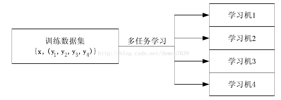
多任务学习（Multi-task learning）

多任务学习（Multi-task learning）是和单任务学习（single-task learning）相对的一种机器学习方法。在机器学习领域，标准的算法理论是一次学习一个任务，也就是系统的输出为实数的情况。复杂的学习问题先被分解成理论上独立的子问题，然后分别对每个子问题进行学习，最后通过对子问题学习结果的组合建立复杂问题的数学模型。多任务学习是一种联合学习，多个任务并行学习，结果相互影响。

拿大家经常使用的school data做个简单的对比，school data是用来预测学生成绩的回归问题的数据集，总共有139个中学的15362个学生，其中每一个中学都可以看作是一个预测任务。单任务学习就是忽略任务之间可能存在的关系分别学习139个回归函数进行分数的预测，或者直接将139个学校的所有数据放到一起学习一个回归函数进行预测。而多任务学习则看重 任务之间的联系，通过联合学习，同时对139个任务学习不同的回归函数，既考虑到了任务之间的差别，又考虑到任务之间的联系，这也是多任务学习最重要的思想之一。

多任务学习早期的研究工作源于对机器学习中的一个重要问题，即“归纳偏置(inductive bias)”问题的研究。机器学习的过程可以看作是对与问题相关的经验数据进行分析，从中归纳出反映问题本质的模型的过程。归纳偏置的作用就是用于指导学习算法如何在模型空间中进行搜索，搜索所得模型的性能优劣将直接受到归纳偏置的影响，而任何一个缺乏归纳偏置的学习系统都不可能进行有效的学习。不同的学习算法(如决策树，神经网络，支持向量机等)具有不同的归纳偏置，人们在解决实际问题时需要人工地确定采用何种学习算法，实际上也就是主观地选择了不同的归纳偏置策略。一个很直观的想法就是，是否可以将归纳偏置的确定过程也通过学习过程来自动地完成，也就是采用“学习如何去学(learning to learn)”的思想。多任务学习恰恰为上述思想的实现提供了一条可行途径，即利用相关任务中所包含的有用信息，为所关注任务的学习提供更强的归纳偏置。

典型方法

目前多任务学习方法大致可以总结为两类，一是不同任务之间共享相同的参数（common parameter），二是挖掘不同任务之间隐藏的共有数据特征（latent feature）。

=================================================================================================

----------------------------------------------------------------我是个人理解分割线---------------------------------------------------------

单任务就是已经是元任务，不能再细划分为多个子任务了，比如中文分词等任务

个人认为的多任务学习是这样的：比如说目前的事件抽取， 子任务1是触发词（trigger）的识别， 子任务2是关系的抽取，对这个事件抽取而言，我们可以使用串行的方法首先识别触发词其次判断触发词和论元之间的关系。也可以采用联合的方法：触发词的识别和关系的判断是同时进行的，两个子任务是相互影响的。

不过这样理解的话与上面的概念有偏差，待确认。

========================================================================================================

 

Multi-task learning（多任务学习）简介

标签： machine learningmulti-task learning

2014-08-07 21:30  5918人阅读  评论(0)  收藏  举报

 分类：

Multi-task learning

版权声明：本文为博主原创文章，未经博主允许不得转载。

1. 什么是Multi-task learning？

Multi-tasklearning （多任务学习）是和single-task learning （单任务学习）相对的一种机器学习方法。拿大家经常使用的school data做个简单的对比，school data是用来预测学生成绩的回归问题的数据集，总共有139个中学的15362个学生，其中每一个中学都可以看作是一个预测任务。单任务学习就是忽略任务之间可能存在的关系分别学习139个回归函数进行分数的预测，或者直接将139个学校的所有数据放到一起学习一个回归函数进行预测。而多任务学习则看重任务之间的联系，通过联合学习，同时对139个任务学习不同的回归函数，既考虑到了任务之间的差别，又考虑到任务之间的联系，这也是多任务学习最重要的思想之一。

 

2. Multi-task learning的优势

Multi-tasklearning的研究也有大概20年之久，虽然没有单任务学习那样受关注，但是也不时有不错的研究成果出炉，与单任务学习相比，多任务学习的优势在哪呢？上节我们已经提到了单任务学习的过程中忽略了任务之间的联系，而现实生活中的学习任务往往是有千丝万缕的联系的，比如多标签图像的分类，人脸的识别等等，这些任务都可以分为多个子任务去学习，多任务学习的优势就在于能发掘这些子任务之间的关系，同时又能区分这些任务之间的差别。

 

3. Multi-tasklearning的学习方法

目前多任务学习方法大致可以总结为两类，一是不同任务之间共享相同的参数（common parameter），二是挖掘不同任务之间隐藏的共有数据特征（latent feature）。下面将简单介绍几篇比较经典的多任务学习的论文及算法思想。

A. Regularizedmulti-task learning

这篇文章很有必要一看，文中提出了基于最小正则化方程的多任务学习方法，并以SVM为例给出多任务学习支持向量机，将多任务学习与经典的单任务学习SVM联系在一起，并给出了详细的求解过程和他们之间的联系，当然实验结果也证明了多任务支持向量机的优势。文中最重要的假设就是所有任务的分界面共享一个中心分界面，然后再次基础上平移，偏移量和中心分界面最终决定了当前任务的分界面。

 

B. Convex multi-taskfeature learning

本文也是一篇典型的多任务学习模型，并且是典型的挖掘多任务之间共有特征的多任务模型，文中给出了多任务特征学习的一个框架，也成为后来许多多任务学习参考的基础。

 

C. Multitasksparsity via maximum entropy discrimination

这篇文章可以看作是比较全面的总结性文章，文中总共讨论了四种情况，feature selection, kernel selection,adaptive pooling and graphical model structure。并详细介绍了四种多任务学习方法，很具有参考价值。

本文只是对多任务学习做了简单的介绍，想要深入了解的话，建议大家看看上面提到的论文。

 

Reference

[1] T. Evgeniouand M. Pontil. Regularized multi-task learning. In Proceeding of thetenth ACM SIGKDD international conference on Knowledge Discovery and DataMining, 2004.

[2] T. Jebara. MultitaskSparsity via Maximum Entropy Discrimination. In Journal of Machine LearningResearch, (12):75-110, 2011.

[3] A. Argyriou,T. Evgeniou and M. Pontil. Convex multitask feature learning. In MachineLearning, 73(3):243-272, 2008.

中国科学技术大学多媒体计算与通信教育部-微软重点实验室  

                                                                                                                      MultiMedia Computing Group

=====================================================================================

Multi-task learning

From Wikipedia, the free encyclopedia

Multi-task learning (MTL) is a subfield of machine learning in which multiple learning tasks are solved at the same time, while exploiting commonalities and differences across tasks. This can result in improved learning efficiency and prediction accuracy for the task-specific models, when compared to training the models separately.^[1][2][3]

In a widely cited 1997 paper, Rich Caruana gave the following characterization:

Multitask Learning is an approach to inductive transfer that improves generalization by using the domain information contained in the training signals of related tasks as an inductive bias. It does this by learning tasks in parallel while using a shared representation; what is learned for each task can help other tasks be learned better.^[3]

In the classification context, MTL aims to improve the performance of multiple classification tasks by learning them jointly. One example is a spam-filter, which can be treated as distinct but related classification tasks across different users. To make this more concrete, consider that different people have different distributions of features which distinguish spam emails from legitimate ones, for example an English speaker may find that all emails in Russian are spam, not so for Russian speakers. Yet there is a definite commonality in this classification task across users, for example one common feature might be text related to money transfer. Solving each user's spam classification problem jointly via MTL can let the solutions inform each other and improve performance.^[4] Further examples of settings for MTL include multiclass classification and multi-label classification.^[5]

Multi-task learning works because regularization induced by requiring an algorithm to perform well on a related task can be superior to regularization that prevents overfitting by penalizing all complexity uniformly. One situation where MTL may be particularly helpful is if the tasks share significant commonalities and are generally slightly under sampled.^[4] However, as discussed below, MTL has also been shown to be beneficial for learning unrelated tasks.^[6]

Methods[edit]

Task grouping and overlap[edit]

Within the MTL paradigm, information can be shared across some or all of the tasks. Depending on the structure of task relatedness, one may want to share information selectively across the tasks. For example, tasks may be grouped or exist in a hierarchy, or be related according to some general metric. Suppose, as developed more formally below, that the parameter vector modeling each task is a linear combination of some underlying basis. Similarity in terms of this basis can indicate the relatedness of the tasks. For example with sparsity, overlap of nonzero coefficients across tasks indicates commonality. A task grouping then corresponds to those tasks lying in a subspace generated by some subset of basis elements, where tasks in different groups may be disjoint or overlap arbitrarily in terms of their bases.^[7] Task relatedness can be imposed a priori or learned from the data.^[5][8]

Exploiting unrelated tasks[edit]

One can attempt learning a group of principal tasks using a group of auxiliary tasks, unrelated to the principal ones. In many applications, joint learning of unrelated tasks which use the same input data can be beneficial. The reason is that prior knowledge about task relatedness can lead to sparser and more informative representations for each task grouping, essentially by screening out idiosyncrasies of the data distribution. Novel methods which builds on a prior multitask methodology by favoring a shared low-dimensional representation within each task grouping have been proposed. The programmer can impose a penalty on tasks from different groups which encourages the two representations to be orthogonal. Experiments on synthetic and real data have indicated that incorporating unrelated tasks can result in significant improvements over standard multi-task learning methods.^[6]

Transfer of knowledge[edit]

Related to multi-task learning is the concept of knowledge transfer. Whereas traditional multi-task learning implies that a shared representation is developed concurrently across tasks, transfer of knowledge implies a sequentially shared representation. Large scale machine learning projects such as the deep convolutional neural network GoogLeNet,^[9] an image-based object classifier, can develop robust representations which may be useful to further algorithms learning related tasks. For example, the pre-trained model can be used as a feature extractor to perform pre-processing for another learning algorithm. Or the pre-trained model can be used to initialize a model with similar architecture which is then fine-tuned to learn a different classification task.^[10]

Mathematics[edit]

Reproducing Hilbert space of vector valued functions (RKHSvv)[edit]

The MTL problem can be cast within the context of RKHSvv (a complete inner product space of vector-valued functions equipped with a reproducing kernel). In particular, recent focus has been on cases where task structure can be identified via a separable kernel, described below. The presentation here derives from Ciliberto et al, 2015.^[5]

RKHSvv concepts[edit]

Suppose the training data set is {\displaystyle {\mathcal {S}}_{t}=\{(x_{i}^{t},y_{i}^{t})\}_{i=1}^{n_{t}}}, with {\displaystyle x_{i}^{t}\in {\mathcal {X}}}, {\displaystyle y_{i}^{t}\in {\mathcal {Y}}}, where {\displaystyle t} indexes task, and {\displaystyle t\in 1,...,T}. Let {\displaystyle n=\sum _{t=1}^{T}n_{t}}. In this setting there is a consistent input and output space and the same loss function {\displaystyle {\mathcal {L}}:\mathbb {R} \times \mathbb {R} \rightarrow \mathbb {R} _{+}} for each task: . This results in the regularized machine learning problem:

{\displaystyle \min _{f\in {\mathcal {H}}}\sum _{t=1}^{T}{\frac {1}{n_{t}}}\sum _{i=1}^{n_{t}}{\mathcal {L}}(y_{i}^{t},f_{t}(x_{i}^{t}))+\lambda ||f||_{\mathcal {H}}^{2}}

(1)

where {\displaystyle {\mathcal {H}}} is a vector valued reproducing kernel Hilbert space with functions {\displaystyle f:{\mathcal {X}}\rightarrow {\mathcal {Y}}^{T}} having components {\displaystyle f_{t}:{\mathcal {X}}\rightarrow {\mathcal {Y}}}.

The reproducing kernel for the space {\displaystyle {\mathcal {H}}} of functions {\displaystyle f:{\mathcal {X}}\rightarrow \mathbb {R} ^{T}} is a symmetric matrix-valued function {\displaystyle \Gamma :{\mathcal {X}}\times {\mathcal {X}}\rightarrow \mathbb {R} ^{T\times T}} , such that {\displaystyle \Gamma (\cdot ,x)c\in {\mathcal {H}}} and the following reproducing property holds:

{\displaystyle \langle f(x),c\rangle _{\mathbb {R} ^{T}}=\langle f,\Gamma (x,\cdot )c\rangle _{\mathcal {H}}}

(2)

The reproducing kernel gives rise to a representer theorem showing that any solution to equation 1 has the form:

{\displaystyle f(x)=\sum _{t=1}^{T}\sum _{i=1}^{n_{t}}\Gamma (x,x_{i}^{t})c_{i}^{t}}

(3)

Separable kernels[edit]

The form of the kernel {\displaystyle \Gamma } induces both the representation of the feature space and structures the output across tasks. A natural simplification is to choose a separable kernel, which factors into separate kernels on the input space {\displaystyle {\mathcal {X}}}and on the tasks {\displaystyle \{1,...,T\}}. In this case the kernel relating scalar components {\displaystyle f_{t}} and {\displaystyle f_{s}} is given by {\textstyle \gamma ((x_{i},t),(x_{j},s))=k(x_{i},x_{j})k_{T}(s,t)=k(x_{i},x_{j})A_{s,t}}. For vector valued functions {\displaystyle f\in {\mathcal {H}}} we can write {\displaystyle \Gamma (x_{i},x_{j})=k(x_{i},x_{j})A}, where {\displaystyle k} is a scalar reproducing kernel, and {\displaystyle A} is a symmetric positive semi-definite {\displaystyle T\times T} matrix. Henceforth denote {\displaystyle S_{+}^{T}=\{{\text{PSD matrices}}\}\subset \mathbb {R} ^{T\times T}} .

This factorization property, separability, implies the input feature space representation does not vary by task. That is, there is no interaction between the input kernel and the task kernel. The structure on tasks is represented solely by {\displaystyle A}. Methods for non-separable kernels {\displaystyle \Gamma } is an current field of research.

For the separable case, the representation theorem is reduced to {\textstyle f(x)=\sum _{i=1}^{N}k(x,x_{i})Ac_{i}}. The model output on the training data is then {\displaystyle KCA} , where {\displaystyle K} is the {\displaystyle n\times n} empirical kernel matrix with entries {\textstyle K_{i,j}=k(x_{i},x_{j})}, and {\displaystyle C} is the {\displaystyle n\times T} matrix of rows {\displaystyle c_{i}}.

With the separable kernel, equation 1 can be rewritten as

{\displaystyle \min _{C\in \mathbb {R} ^{n\times T}}V(Y,KCA)+\lambda tr(KCAC^{\top })}

(P)

where {\displaystyle V} is a (weighted) average of {\displaystyle {\mathcal {L}}} applied entry-wise to Y and KCA. (The weight is zero if {\displaystyle Y_{i}^{t}} is a missing observation).

Note the second term in P can be derived as follows:

{\displaystyle ||f||_{\mathcal {H}}^{2}=\langle \sum _{i=1}^{n}k(\cdot ,x_{i})Ac_{i},\sum _{j=1}^{n}k(\cdot ,x_{j})Ac_{j}\rangle _{\mathcal {H}}}

{\displaystyle =\sum _{i,j=1}^{n}\langle k(\cdot ,x_{i})Ac_{i},k(\cdot ,x_{j})Ac_{j}\rangle _{\mathcal {H}}} (bilinearity)

{\displaystyle =\sum _{i,j=1}^{n}\langle k(x_{i},x_{j})Ac_{i},c_{j}\rangle _{\mathbb {R} ^{T}}} (reproducing property)

{\displaystyle =\sum _{i,j=1}^{n}k(x_{i},x_{j})c_{i}^{\top }Ac_{j}=tr(KCAC^{\top })}

Known task structure[edit]

Task structure representations[edit]

There are three largely equivalent ways to represent task structure: through a regularizer; through an output metric, and through an output mapping.

Regularizer - With the separable kernel, it can be shown (below) that {\textstyle ||f||_{\mathcal {H}}^{2}=\sum _{s,t=1}^{T}A_{t,s}^{\dagger }\langle f_{s},f_{t}\rangle _{{\mathcal {H}}_{k}}}, where {\displaystyle A_{t,s}^{\dagger }} is the {\displaystyle t,s} element of the pseudoinverse of {\displaystyle A}, and {\displaystyle {\mathcal {H}}_{k}} is the RKHS based on the scalar kernel {\displaystyle k}, and {\textstyle f_{t}(x)=\sum _{i=1}^{n}k(x,x_{i})A_{t}^{\top }c_{i}}. This formulation shows that {\displaystyle A_{t,s}^{\dagger }} controls the weight of the penalty associated with {\textstyle \langle f_{s},f_{t}\rangle _{{\mathcal {H}}_{k}}}. (Note that {\textstyle \langle f_{s},f_{t}\rangle _{{\mathcal {H}}_{k}}} arises from {\textstyle ||f_{t}||_{{\mathcal {H}}_{k}}=\langle f_{t},f_{t}\rangle _{{\mathcal {H}}_{k}}}.)

Proof:

{\displaystyle ||f||_{\mathcal {H}}^{2}=\langle \sum _{i=1}^{n}\gamma ((x_{i},t_{i}),\cdot )c_{i}^{t_{i}},\sum _{j=1}^{n}\gamma ((x_{j},t_{j}),\cdot )c_{j}^{t_{j}}\rangle _{\mathcal {H}}}

{\displaystyle =\sum _{i,j=1}^{n}c_{i}^{t_{i}}c_{j}^{t_{j}}\gamma ((x_{i},t_{i}),(x_{j},t_{j}))}

{\displaystyle =\sum _{i,j=1}^{n}\sum _{s,t=1}^{T}c_{i}^{t}c_{j}^{s}k(x_{i},x_{j})A_{s,t}}

{\displaystyle =\sum _{i,j=1}^{n}k(x_{i},x_{j})\langle c_{i},Ac_{j}\rangle _{\mathbb {R} ^{T}}}

{\displaystyle =\sum _{i,j=1}^{n}k(x_{i},x_{j})\langle c_{i},AA^{\dagger }Ac_{j}\rangle _{\mathbb {R} ^{T}}}

{\displaystyle =\sum _{i,j=1}^{n}k(x_{i},x_{j})\langle Ac_{i},A^{\dagger }Ac_{j}\rangle _{\mathbb {R} ^{T}}}

{\displaystyle =\sum _{i,j=1}^{n}\sum _{s,t=1}^{T}(Ac_{i})^{t}(Ac_{j})^{s}k(x_{i},x_{j})A_{s,t}^{\dagger }}

{\displaystyle =\sum _{s,t=1}^{T}A_{s,t}^{\dagger }\langle \sum _{i=1}^{n}k(x_{i},\cdot )(Ac_{i})^{t},\sum _{j=1}^{n}k(x_{j},\cdot )(Ac_{j})^{s}\rangle _{{\mathcal {H}}_{k}}}

{\displaystyle =\sum _{s,t=1}^{T}A_{s,t}^{\dagger }\langle f_{t},f_{s}\rangle _{{\mathcal {H}}_{k}}}

Output metric - an alternative output metric on {\displaystyle {\mathcal {Y}}^{T}} can be induced by the inner product {\displaystyle \langle y_{1},y_{2}\rangle _{\Theta }=\langle y_{1},\Theta y_{2}\rangle _{\mathbb {R} ^{T}}}. With the squared loss there is an equivalence between the separable kernels {\displaystyle k(\cdot ,\cdot )I_{T}} under the alternative metric, and {\displaystyle k(\cdot ,\cdot )\Theta }, under the canonical metric.

Output mapping - Outputs can be mapped as {\displaystyle L:{\mathcal {Y}}^{T}\rightarrow {\mathcal {\tilde {Y}}}} to a higher dimensional space to encode complex structures such as trees, graphs and strings. For linear maps {\displaystyle L}, with appropriate choice of separable kernel, it can be shown that{\displaystyle A=L^{\top }L}.

Task structure examples[edit]

Via the regularizer formulation, one can represent a variety of task structures easily.

• Letting {\textstyle A^{\dagger }=\gamma I_{T}+(\gamma -\lambda ){\frac {1}{T}}{\mathbf {1}}{\mathbf {1}}^{\top }} (where {\displaystyle I_{T}} is the TxT identity matrix, and {\textstyle {\mathbf {1}}{\mathbf {1}}^{\top }} is the TxT matrix of ones) is equivalent to letting {\displaystyle \gamma } control the variance {\textstyle \sum _{t}||f_{t}-{\bar {f}}||_{{\mathcal {H}}_{k}}} of tasks from their mean {\textstyle {\frac {1}{T}}\sum _{t}f_{t}}. For example, blood levels of some biomarker may be taken on {\displaystyle T} patients at {\displaystyle n_{t}} time points during the course of a day and interest may lie in regularizing the variance of the predictions across patients.
• Letting {\displaystyle A^{\dagger }=\alpha I_{T}+(\alpha -\lambda )M} , where {\displaystyle M_{t,s}={\frac {1}{|G_{r}|}}\mathbb {I} (t,s\in G_{r})} is equivalent to letting {\displaystyle \alpha } control the variance measured with respect to a group mean: {\displaystyle \sum _{r}\sum _{t\in G_{r}}||f_{t}-{\frac {1}{|G_{r}|}}\sum _{s\in G_{r})}f_{s}||}. (Here {\displaystyle |G_{r}|} the cardinality of group r, and {\displaystyle \mathbb {I} } is the indicator function). For example people in different political parties (groups) might be regularized together with respect to predicting the favorability rating of a politician. Note that this penalty reduces to the first when all tasks are in the same group.
• Letting {\displaystyle A^{\dagger }=\delta I_{T}+(\delta -\lambda )L}, where {\displaystyle L=D-M} is the Laplacian for the graph with adjacency matrix M giving pairwise similarities of tasks. This is equivalent to giving a larger penalty to the distance separating tasks t and s when they are more similar (according to the weight {\displaystyle M_{t,s}},) i.e. {\displaystyle \delta } regularizes {\displaystyle \sum _{t,s}||f_{t}-f_{s}||_{{\mathcal {H}}_{k}}^{2}M_{t,s}}.
• All of the above choices of A also induce the additional regularization term {\textstyle \lambda \sum _{t}||f||_{{\mathcal {H}}_{k}}^{2}} which penalizes complexity in f more broadly.

Learning tasks together with their structure[edit]

Learning problem P can be generalized to admit learning task matrix A as follows:

{\displaystyle \min _{C\in \mathbb {R} ^{n\times T},A\in S_{+}^{T}}V(Y,KCA)+\lambda tr(KCAC^{\top })+F(A)}

(Q)

Choice of {\displaystyle F:S_{+}^{T}\rightarrow \mathbb {R} _{+}} must be designed to learn matrices A of a given type. See "Special cases" below.

Optimization of Q[edit]

Restricting to the case of convex losses and coercive penalties Ciliberto et al have shown that although Q is not convex jointly in C and A, a related problem is jointly convex.

Specifically on the convex set {\displaystyle {\mathcal {C}}=\{(C,A)\in \mathbb {R} ^{n\times T}\times S_{+}^{T}|Range(C^{\top }KC)\subseteq Range(A)\}}, the equivalent problem

{\displaystyle \min _{C,A\in {\mathcal {C}}}V(Y,KC)+\lambda tr(A^{\dagger }C^{\top }KC)+F(A)}

(R)

is convex with the same minimum value. And if {\displaystyle (C_{R},A_{R})} is a minimizer for R then {\displaystyle (C_{R}A_{R}^{\dagger },A_{R})} is a minimizer for Q.

R may be solved by a barrier method on a closed set by introducing the following perturbation:

{\displaystyle \min _{C\in \mathbb {R} ^{n\times T},A\in S_{+}^{T}}V(Y,KC)+\lambda tr(A^{\dagger }(C^{\top }KC+\delta ^{2}I_{T}))+F(A)}

(S)

The perturbation via the barrier {\displaystyle \delta ^{2}tr(A^{\dagger })} forces the objective functions to be equal to {\displaystyle +\infty } on the boundary of {\displaystyle R^{n\times T}\times S_{+}^{T}} .

S can be solved with a block coordinate descent method, alternating in C and A. This results in a sequence of minimizers {\displaystyle (C_{m},A_{m})} in S that converges to the solution in R as {\displaystyle \delta _{m}\rightarrow 0}, and hence gives the solution to Q.

Special cases[edit]

Spectral penalties - Dinnuzo et al^[11] suggested setting F as the Frobenius norm {\displaystyle {\sqrt {tr(A^{\top }A)}}}. They optimized Q directly using block coordinate descent, not accounting for difficulties at the boundary of {\displaystyle \mathbb {R} ^{n\times T}\times S_{+}^{T}}.

Clustered tasks learning - Jacob et al^[12] suggested to learn A in the setting where T tasks are organized in R disjoint clusters. In this case let {\displaystyle E\in \{0,1\}^{T\times R}} be the matrix with {\displaystyle E_{t,r}=\mathbb {I} ({\text{task }}t\in {\text{group }}r)}. Setting {\displaystyle M=I-E^{\dagger }E^{T}}, and{\displaystyle U={\frac {1}{T}}{\mathbf {11}}^{\top }}, the task matrix {\displaystyle A^{\dagger }} can be parameterized as a function of {\displaystyle M}: {\displaystyle A^{\dagger }(M)=\epsilon _{M}U+\epsilon _{B}(M-U)+\epsilon (I-M)} , with terms that penalize the average, between clusters variance and within clusters variance respectively of the task predictions. M is not convex, but there is a convex relaxation {\displaystyle {\mathcal {S}}_{c}=\{M\in S_{+}^{T}:I-M\in S_{+}^{T}\land tr(M)=r\}}. In this formulation, {\displaystyle F(A)=\mathbb {I} (A(M)\in \{A:M\in {\mathcal {S}}_{C}\})}.

Generalizations[edit]

Non-convex penalties - Penalties can be constructed such that A is constrained to be a graph Laplacian, or that A has low rank factorization. However these penalties are not convex, and the analysis of the barrier method proposed by Ciliberto et al does not go through in these cases.

Non-separable kernels - Separable kernels are limited, in particular they do not account for structures in the interaction space between the input and output domains jointly. Future work is needed to develop models for these kernels.

Applications[edit]

Spam filtering[edit]

Using the principles of MTL, techniques for collaborative spam filtering that facilitates personalization have been proposed. In large scale open membership email systems, most users do not label enough messages for an individual local classifier to be effective, while the data is too noisy to be used for a global filter across all users. A hybrid global/individual classifier can be effective at absorbing the influence of users who label emails very diligently from the general public. This can be accomplished while still providing sufficient quality to users with few labeled instances.^[13]

Web search[edit]

Using boosted decision trees, one can enable implicit data sharing and regularization. This learning method can be used on web-search ranking data sets. One example is to use ranking data sets from several countries. Here, multitask learning is particularly helpful as data sets from different countries vary largely in size because of the cost of editorial judgments. It has been demonstrated that learning various tasks jointly can lead to significant improvements in performance with surprising reliability.^[14]

RoboEarth[edit]

In order to facilitate transfer of knowledge, IT infrastructure is being developed. One such project, RoboEarth, aims to set up an open source internet database that can be accessed and continually updated from around the world. The goal is to facilitate a cloud-based interactive knowledge base, accessible to technology companies and academic institutions, which can enhance the sensing, acting and learning capabilities of robots and other artificial intelligence agents.^[15]

Software package[edit]

The Multi-Task Learning via StructurAl Regularization (MALSAR) Matlab package ^[16] implements the following multi-task learning algorithms:

• Mean-Regularized Multi-Task Learning^[17][18]
• Multi-Task Learning with Joint Feature Selection^[19]
• Robust Multi-Task Feature Learning^[20]
• Trace-Norm Regularized Multi-Task Learning^[21]
• Alternating Structural Optimization^[22][23]
• Incoherent Low-Rank and Sparse Learning^[24]
• Robust Low-Rank Multi-Task Learning
• Clustered Multi-Task Learning^[25][26]
• Multi-Task Learning with Graph Structures

See also[edit]

• Artificial Intelligence
• Artificial neural network
• Evolutionary computation
• Human-based genetic algorithm
• Kernel methods for vector output
• Machine Learning
• Robotics

References[edit]

1. Jump up^ Baxter, J. (2000). A model of inductive bias learning. Journal of Artificial Intelligence Research, 12:149--198, On-line paper
2. Jump up^ Thrun, S. (1996). Is learning the n-th thing any easier than learning the first?. In Advances in Neural Information Processing Systems 8, pp. 640--646. MIT Press. Paper at Citeseer
3. ^ Jump up to:^a b Caruana, R. (1997). "Multi-task learning" (PDF). Machine Learning. doi:10.1023/A:1007379606734.
4. ^ Jump up to:^a b Weinberger, Kilian. "Multi-task Learning".
5. ^ Jump up to:^a b c Ciliberto, C. (2015). "Convex Learning of Multiple Tasks and their Structure". arXiv:1504.03101.
6. ^ Jump up to:^a b Romera-Paredes, B., Argyriou, A., Bianchi-Berthouze, N., & Pontil, M., (2012) Exploiting Unrelated Tasks in Multi-Task Learning. http://jmlr.csail.mit.edu/proceedings/papers/v22/romera12/romera12.pdf
7. Jump up^ Kumar, A., & Daume III, H., (2012) Learning Task Grouping and Overlap in Multi-Task Learning. http://icml.cc/2012/papers/690.pdf
8. Jump up^ Jawanpuria, P., & Saketha Nath, J., (2012) A Convex Feature Learning Formulation for Latent Task Structure Discovery. http://icml.cc/2012/papers/90.pdf
9. Jump up^ Szegedy, C. (2014). "Going Deeper with Convolutions". Computer Vision and Pattern Recognition (CVPR), 2015 IEEE Conference on. arXiv:1409.4842. doi:10.1109/CVPR.2015.7298594.
10. Jump up^ Roig, Gemma. "Deep Learning Overview" (PDF).
11. Jump up^ Dinuzzo, Francesco (2011). "Learning output kernels with block coordinate descent.". Proceedings of the 28th International Conference on Machine Learning (ICML-11).
12. Jump up^ Jacob, Laurent (2009). "Clustered multi-task learning: A convex formulation". Advances in neural information processing systems.
13. Jump up^ Attenberg, J., Weinberger, K., & Dasgupta, A. Collaborative Email-Spam Filtering with the Hashing-Trick. http://www.cse.wustl.edu/~kilian/papers/ceas2009-paper-11.pdf
14. Jump up^ Chappelle, O., Shivaswamy, P., & Vadrevu, S. Multi-Task Learning for Boosting with Application to Web Search Ranking. http://www.cse.wustl.edu/~kilian/papers/multiboost2010.pdf
15. Jump up^ Description of RoboEarth Project
16. Jump up^ Zhou, J., Chen, J. and Ye, J. MALSAR: Multi-tAsk Learning via StructurAl Regularization. Arizona State University, 2012. http://www.public.asu.edu/~jye02/Software/MALSAR. On-line manual
17. Jump up^ Evgeniou, T., & Pontil, M. (2004). Regularized multi–task learning. Proceedings of the tenth ACM SIGKDD international conference on Knowledge discovery and data mining (pp. 109–117).
18. Jump up^ Evgeniou, T., Micchelli, C., & Pontil, M. (2005). Learning multiple tasks with kernel methods. Journal of Machine Learning Research, 6, 615.
19. Jump up^ Argyriou, A., Evgeniou, T., & Pontil, M. (2008a). Convex multi-task feature learning. Machine Learning, 73, 243–272.
20. Jump up^ Chen, J., Zhou, J., & Ye, J. (2011). Integrating low-rank and group-sparse structures for robust multi-task learning. Proceedings of the tenth ACM SIGKDD international conference on Knowledge discovery and data mining.
21. Jump up^ Ji, S., & Ye, J. (2009). An accelerated gradient method for trace norm minimization. Proceedings of the 26th Annual International Conference on Machine Learning (pp. 457–464).
22. Jump up^ Ando, R., & Zhang, T. (2005). A framework for learning predictive structures from multiple tasks and unlabeled data. The Journal of Machine Learning Research, 6, 1817–1853.
23. Jump up^ Chen, J., Tang, L., Liu, J., & Ye, J. (2009). A convex formulation for learning shared structures from multiple tasks. Proceedings of the 26th Annual International Conference on Machine Learning (pp. 137–144).
24. Jump up^ Chen, J., Liu, J., & Ye, J. (2010). Learning incoherent sparse and low-rank patterns from multiple tasks. Proceedings of the 16th ACM SIGKDD international conference on Knowledge discovery and data mining (pp. 1179–1188).
25. Jump up^ Jacob, L., Bach, F., & Vert, J. (2008). Clustered multi-task learning: A convex formulation. Advances in Neural Information Processing Systems， 2008
26. Jump up^ Zhou, J., Chen, J., & Ye, J. (2011). Clustered multi-task learning via alternating structure optimization. Advances in Neural Information Processing Systems.