【吴恩达深度学习编程作业】1.2神经网络基础——识别猫的程序

很早之前就学完深度学习第二周的课程，由于保研的事情一直心烦，做什么事情都索然无味，还有七天出结果，今天终于沉下心把剩余的部分跟着blog具有神经网络思维的Logistic回归码了一遍，老师课程讲的很清楚，自己也做了笔记，但是编程作业中还是有些语句不理解，下面贴出自己的源码和运行结果：

lr_utils.py文件

import numpy as np
import h5py
    
    
def load_dataset():
    train_dataset = h5py.File('datasets/train_catvnoncat.h5', "r")
    # 保存训练集里的图像数据（本训练集有209张64×64的图像）
    train_set_x_orig = np.array(train_dataset["train_set_x"][:]) # your train set features
    # 保存训练集的图像对应的分类值（【0|1】0表示不是猫，1表示是猫）
    train_set_y_orig = np.array(train_dataset["train_set_y"][:]) # your train set labels

    test_dataset = h5py.File('datasets/test_catvnoncat.h5', "r")
    # 保存测试集里的图像数据（本训练集有50张64×64的图像）
    test_set_x_orig = np.array(test_dataset["test_set_x"][:]) # your test set features
    # 保存测试集的图像对应的分类值（【0|1】0表示不是猫，1表示是猫 ）
    test_set_y_orig = np.array(test_dataset["test_set_y"][:]) # your test set labels

    # 保存的是以bytes类型保存的两个字符串数据，数据位：
    classes = np.array(test_dataset["list_classes"][:]) # the list of classes
    
    train_set_y_orig = train_set_y_orig.reshape((1, train_set_y_orig.shape[0]))
    test_set_y_orig = test_set_y_orig.reshape((1, test_set_y_orig.shape[0]))
    
    return train_set_x_orig, train_set_y_orig, test_set_x_orig, test_set_y_orig, classes

main.py文件

# 搭建一个可以识别猫的神经网络

import matplotlib.pyplot as plt
import numpy as np
from Deep_Learning.lr_utils import load_dataset   # 加载资料包里面的数据的简单功能的库

# 把数据加载到主程序中
train_set_x_orig, train_set_y, test_set_x_orig, test_set_y, classes = load_dataset()
# 查看训练集里的第26张图片
index = 15
plt.imshow(train_set_x_orig[index])
plt.waitforbuttonpress()
# 查看训练集里的标签
print("train_set_y" + str(train_set_y))

# 打印当前训练集的标签值
# 使用np.squeeze的目的是压缩维度，【未压缩】train_set_y[:,index]的值为[1]，【压缩后】np.squeeze(train_set_y[:,index])的值为[1]
print("使用np.squeeze" + str(np.squeeze(train_set_y[:, index])) + ",不使用np.squeeze" + str(train_set_y[:, index]))
print("y=" + str(train_set_y[:, index]) + ",it`s a " + classes[np.squeeze(train_set_y[:, index])].decode("utf-8") + "' picture")

m_train = train_set_y.shape[1]  # 训练集里图片数量
m_test = test_set_y.shape[1]    # 测试集里图片的数量
# train_set_x_orig是一个维度为（m_train,num_px,num_px,3）的数组
num_px = train_set_x_orig.shape[1]  # 训练、测试集里的图片宽度和高度（均为64×64）

# 查看加载的具体情况
print("训练集的数量：m_train = " + str(m_train))
print("测试集的数量：m_test = " + str(m_test))
print("每张图片的宽/高：num_px = " + str(num_px))
print("每张图片的大小：(" + str(num_px) + "," + str(num_px) + ",3)")
print("训练集_图片的维度：" + str(train_set_x_orig.shape))
print("训练集_标签的维度: " + str(train_set_y.shape))
print("测试集_图片的维度：" + str(test_set_x_orig.shape))
print("测试集_标签的维度: " + str(test_set_y.shape))

# 为了方便，把维度为（64,64,3）的numpy数组重构为（64×64×3,1）的数组，若想将形状（a,b,c,d）的矩阵平铺为形状（b*c*d,a）的矩阵可使用以下代码
# 将训练集的维度降低并转置
train_set_x_flatten = train_set_x_orig.reshape(train_set_x_orig.shape[0], -1).T  # 其中-1是指不确定是哪一列，若参数为1则为第一列
# 将测试集的围兜降低并转置
test_set_x_flatten = test_set_x_orig.reshape(test_set_x_orig.shape[0], -1).T

# 查看降维之后的具体情况
print("训练集降维之后的维度：" + str(train_set_x_flatten.shape))
print("测试集降维之后的维度：" + str(test_set_x_flatten.shape))

# 标准化数据集，数据集每一行除以255（像素通道的最大值），让标准化的数据位于[0,1]之间
train_set_x = train_set_x_flatten / 255
test_set_x = test_set_x_flatten / 255


# 构建sigmoid函数
def sigmoid(z):
    return 1 / (1 + np.exp(-z))
#  测试sigmoid()
print("=========测试sigmoid=========")
print("sigmoid(0) = " + str(sigmoid(0)))

# 初始化参数w和b
def initialize_with_zeros(dim):
    """
        此函数为w创建一个维度为（dim,1）的0向量，并将b初始化为0
    :param dim:     -我们想要的w矢量的大小（或者这种情况下的参数数量）
    :return:    w   -维度为（dim,1）的初始化向量
                b   -初始化的标量（对应于偏差）
    """
    w = np.zeros(shape=(dim, 1))
    b = 0
    # 使用断言确保数据的正确性
    assert (w.shape == (dim, 1))     # w的维度是（dim,1）
    assert (isinstance(b, float) or isinstance(b, int))    # b的类型是float或者int
    return (w, b)

def propagate(w, b, X, Y):
    """
    实现前向和后向传播的成本函数及其梯度
    :param w:   -权重，大小不等的数组（num_px * num_px * 3,1）
    :param b:   -偏差，一个标量
    :param X:   -矩阵类型为（num_px * num_px * 3,训练数量）
    :param Y:   -真正的"标签"矢量（如果非猫则为0，是猫则是1），矩阵的维度为（1，训练数据数量）
    :return:cost    -逻辑回归的负对数似然成本
            dw      -相对于w的损失梯度，因此与w是相同的形状
            db      -相对于b的损失梯度，因此与b是相同的形状
    """
    m = X.shape[1]

    # 正向传播
    A = sigmoid(np.dot(w.T, X) + b)     # 计算激活值
    cost = (-1 / m) * np.sum(Y * np.log(A) + (1 - Y) * (np.log(1 - A)))     # 计算成本

    # 反向传播
    dw = (1 / m) * np.dot(X, (A - Y).T)
    db = (1 / m) * np.sum(A - Y)

    # 使用断言确保数据的正确性
    assert (dw.shape == w.shape)
    assert (db.dtype == float)
    cost = np.squeeze(cost)
    assert (cost.shape == ())

    # 创建一个字典，保存dw和db
    grads = {
        "dw": dw,
        "db": db
    }
    return (grads, cost)

# 测试propagate
print("=========测试propagate=========")
# 初始化参数
w, b, X, Y = np.array([[1], [2]]), 2, np.array([[1, 2], [3, 4]]), np.array([[1, 0]])
grads, cost = propagate(w, b, X, Y)
print("dw = " + str(grads["dw"]))
print("db = " + str(grads["db"]))
print("cost = " + str(cost))


# 更新参数，通过最小化成本函数J学习w和b
def optimize(w, b, X, Y, num_iterations, learning_rate, print_cost=False):
    """
    通过运行梯度下降算法优化w和b
    :param w:   -权重，大小不等的数组（num_px * num_px * 3,1 ）
    :param b:   -偏差，标量
    :param X:   -矩阵类型为（num_px * num_px * 3,训练数量）
    :param Y:   -真正的"标签"矢量（如果非猫则为0，是猫则是1），矩阵的维度为（1，训练数据数量）
    :param num_iterations:  -优化循环的迭代次数
    :param learning_rate:   -梯度下降更新规则的学习速率
    :param print_cost:      -每100次打印一次损失值
    :return:params  -包含权重w和b的字典
            grads   -包含权重和偏差对于成本函数的梯度的字典
            cost    -优化期间计算的所有成本列表，用于绘制学习曲线

    我们需要写下两个步骤遍历：
        1.计算当前函数的成本和梯度，使用propagate()
        2.使用w和b的梯度下降法更新参数
    """
    costs = []

    for i in range(num_iterations):
        grads, cost = propagate(w, b, X, Y)
        dw = grads["dw"]
        db = grads["db"]
        w = w - learning_rate * dw
        b = b - learning_rate * db
        # 记录成本
        if i % 100 == 0:
            costs.append(cost)
        # 打印成本数据
        if(print_cost) and (i % 100 == 0):
            print("迭代的次数：%i, 误差值： %f" % (i, cost))

    params = {
        "w": w,
        "b": b
    }
    grads = {
        "dw": dw,
        "db": db
    }

    return (params, grads, costs)

# 测试optimize
print("=================测试optimize===============")
w, b, X, Y = np.array([[1], [2]]), 2, np.array([[1, 2], [3, 4]]), np.array([[1, 0]])
params, grads, costs = optimize(w, b, X, Y, num_iterations=200, learning_rate=0.009, print_cost=False)
print("w = " + str(params["w"]))
print("b = " + str(params["b"]))
print("dw = " + str(grads["dw"]))
print("db = " + str(grads["db"]))


# 实现预测函数
def predict(w, b, X):
    """
    使用学习逻辑回归参数logistic (w,b)预测标签是0还是1
    :param w:   -权重，大小不等的数组（num_px * num_px * 3,1 ）
    :param b:   -偏差，标量
    :param X:   -矩阵类型为（num_px * num_px * 3,训练数量）
    :return: Y_prediction   -包含X中所有图片的所有预测【0 | 1】的一个numpy数组（向量）
    """

    m = X.shape[1]  # 图片的数量
    Y_prediction = np.zeros((1, m))
    w = w.reshape(X.shape[0], 1)

    # 预测猫在图片中出现的频率
    A = sigmoid(np.dot(w.T, X) + b)
    for i in range(A.shape[1]):
        # 将概率a[0,i]转换为实际预测p[0,i]
        Y_prediction[0, 1] = 1 if A[0, i] > 0.5 else 0
    assert (Y_prediction.shape == (1, m))
    return Y_prediction

# 测试predict
print("============测试predict===============")
w, b, X, Y = np.array([[1], [2]]), 2, np.array([[1, 2], [3, 4]]), np.array([[1, 0]])
print("prediction = " + str(predict(w, b, X)))


# 将函数整合到model函数中
def model(X_train, Y_train, X_test, Y_test, num_iterations=2000, learning_rate=0.5, print_cost=False):
    """
    通过调用之前实现的函数构建逻辑回归模型
    :param X_train:     -numpy的数组，维度为（num_px * num_px * 3,m_train）的训练集
    :param Y_train:     -numpy的数组，维度为（1,m_train）（矢量）的训练标签集
    :param X_test:      -numpy的数组，维度为（num_px * num_px * 3,m_train）的测试集
    :param Y_test:      -numpy的数组，维度为（1,m_train）（矢量）的测试标签集
    :param num_iterations:      -表示用于优化参数的迭代次数的超参数
    :param learning_rate:       -表示optimize()更新规则中使用的学习速率的超参数
    :param print_cost:          -设置为true以每100次的迭代打印成本
    :return: d      -包含有关模型信息的字典
    """
    w, b = initialize_with_zeros(X_train.shape[0])
    parameters, grads, costs = optimize(w, b, X_train, Y_train, num_iterations, learning_rate, print_cost)

    # 从字典“参数”中检索参数w和b
    w, b = parameters["w"], parameters["b"]

    # 预测测试/训练集的例子
    Y_prediction_train = predict(w, b, X_train)
    Y_prediction_test = predict(w, b, X_test)

    # 打印训练后的准确性
    print("训练集的准确性：", format(100 - np.mean(np.abs(Y_prediction_train - Y_train)) * 100), "%")
    print("测试集的准确性：", format(100 - np.mean(np.abs(Y_prediction_test - Y_test)) * 100), "%")

    d = {
        "costs": costs,
        "Y_prediction_train": Y_prediction_train,
        "Y_prediction_test": Y_prediction_test,
        "w": w,
        "b": b,
        "learning_rate": learning_rate,
        "num_iterations": num_iterations
    }
    return d


# 测试model
print("===================测试model=====================")
# 这里加载的是真实的数据
d = model(train_set_x, train_set_y, test_set_x, test_set_y, num_iterations=2000, learning_rate=0.005, print_cost=True)


# 绘制图
costs = np.squeeze(d['costs'])
plt.plot(costs)
plt.ylabel('cost')
plt.xlabel('iterations (per hundreds)')
plt.title("learning rate =" + str(d["learning_rate"]))
plt.show()


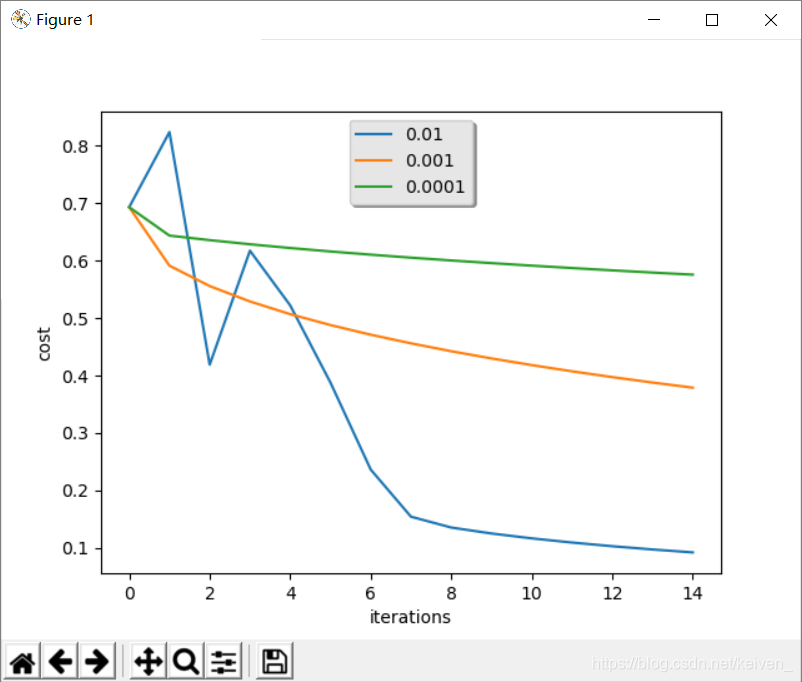
# 比较模型的学习速率和几种学习速率的选择，也可以尝试使用不同于我们初始化的learning_rate变量包含的三个值
learning_rates = [0.01, 0.001, 0.0001]
models = {}
for i in learning_rates:
    print("learning rate is : " + str(i))
    models[str(i)] = model(train_set_x, train_set_y, test_set_x, test_set_y, num_iterations=1500, learning_rate=i, print_cost=False)
    print("\n" + "---------------------------------" + "\n")

for i in learning_rates:
    plt.plot(np.squeeze(models[str(i)]["costs"]), label=str(models[str(i)]["learning_rate"]))
plt.ylabel("cost")
plt.xlabel("iterations")

legend = plt.legend(loc='upper center', shadow=True)
frame = legend.get_frame()
frame.set_facecolor('0.90')
plt.show()

运行结果

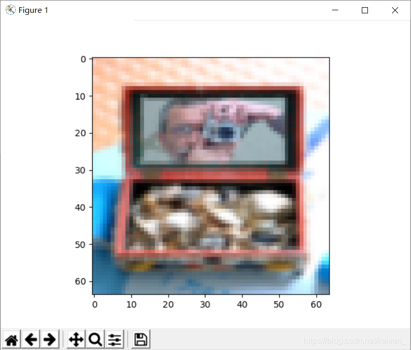
显示第15张图片，这不是猫

当学习速率不同时，迭代次数与代价的关系：

控制台运行结果

train_set_y[[0 0 1 0 0 0 0 1 0 0 0 1 0 1 1 0 0 0 0 1 0 0 0 0 1 1 0 1 0 1 0 0 0 0 0 0
  0 0 1 0 0 1 1 0 0 0 0 1 0 0 1 0 0 0 1 0 1 1 0 1 1 1 0 0 0 0 0 0 1 0 0 1
  0 0 0 0 0 0 0 0 0 0 0 1 1 0 0 0 1 0 0 0 1 1 1 0 0 1 0 0 0 0 1 0 1 0 1 1
  1 1 1 1 0 0 0 0 0 1 0 0 0 1 0 0 1 0 1 0 1 1 0 0 0 1 1 1 1 1 0 0 0 0 1 0
  1 1 1 0 1 1 0 0 0 1 0 0 1 0 0 0 0 0 1 0 1 0 1 0 0 1 1 1 0 0 1 1 0 1 0 1
  0 0 0 0 0 1 0 0 1 0 0 0 1 0 0 0 0 1 0 0 1 0 0 0 0 0 0 0 0]]
使用np.squeeze0,不使用np.squeeze[0]
y=[0],it`s a non-cat' picture
训练集的数量：m_train = 209
测试集的数量：m_test = 50
每张图片的宽/高：num_px = 64
每张图片的大小：(64,64,3)
训练集_图片的维度：(209, 64, 64, 3)
训练集_标签的维度: (1, 209)
测试集_图片的维度：(50, 64, 64, 3)
测试集_标签的维度: (1, 50)
训练集降维之后的维度：(12288, 209)
测试集降维之后的维度：(12288, 50)
=========测试sigmoid=========
sigmoid(0) = 0.5
=========测试propagate=========
dw = [[0.99993216]
 [1.99980262]]
db = 0.49993523062470574
cost = 6.000064773192205
=================测试optimize===============
w = [[-0.25752876]
 [-0.35717757]]
b = 1.4501755960194689
dw = [[0.14547118]
 [0.05636579]]
db = -0.04455269818367541
============测试predict===============
prediction = [[0. 1.]]
===================测试model=====================
迭代的次数：0, 误差值： 0.693147
迭代的次数：100, 误差值： 0.584508
迭代的次数：200, 误差值： 0.466949
迭代的次数：300, 误差值： 0.376007
迭代的次数：400, 误差值： 0.331463
迭代的次数：500, 误差值： 0.303273
迭代的次数：600, 误差值： 0.279880
迭代的次数：700, 误差值： 0.260042
迭代的次数：800, 误差值： 0.242941
迭代的次数：900, 误差值： 0.228004
迭代的次数：1000, 误差值： 0.214820
迭代的次数：1100, 误差值： 0.203078
迭代的次数：1200, 误差值： 0.192544
迭代的次数：1300, 误差值： 0.183033
迭代的次数：1400, 误差值： 0.174399
迭代的次数：1500, 误差值： 0.166521
迭代的次数：1600, 误差值： 0.159305
迭代的次数：1700, 误差值： 0.152667
迭代的次数：1800, 误差值： 0.146542
迭代的次数：1900, 误差值： 0.140872
训练集的准确性： 65.55023923444976 %
测试集的准确性： 34.0 %
learning rate is : 0.01
训练集的准确性： 65.55023923444976 %
测试集的准确性： 34.0 %

---------------------------------

learning rate is : 0.001
训练集的准确性： 65.55023923444976 %
测试集的准确性： 34.0 %

---------------------------------

learning rate is : 0.0001
训练集的准确性： 65.55023923444976 %
测试集的准确性： 34.0 %

---------------------------------