pytorch 数据集处理以及模型训练

守护安静星空

于 2024-02-22 14:04:59 发布

阅读量706

点赞数 12

文章标签： pytorch 人工智能 python

本文链接：https://blog.csdn.net/klp1358484518/article/details/136184190

版权

1.基础类说明

为了统一数据的加载和处理代码，pytorch提供了两个类，用来处理数据加载：

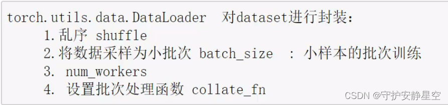
torch.utils.data.DataLoader
torch.utils.data.Dataset

通过这两个类，可以使数据集加载和预处理代码，与模型训练代码脱钩，是代码模块化和可读性更高，DataLoader具有乱序和批次输出的功能非常实用，，以dataset为tensor数据容器，DataLoader可以批量乱序输出dataset容器里面的数据，举例说明DataLoader和TensorDataset（TensorDataset继承自Dataset）。

from torch.utils.data import DataLoader
from torch.utils.data import TensorDataset

#举例使用方法：

x = np.random.randn(100)
y = 100*x+10

x = torch.from_numpy(x)
y = torch.from_numpy(y)

ds = TensorDataset(x,y)
print(ds)
dl = DataLoader(ds,batch_size=10)
print(dl)
for a,s in dl:
	print(a,s)
#x,y = next(iter(s))#使用迭代方式访问
'''
打印输出
<torch.utils.data.dataset.TensorDataset object at 0x000001C25C8B0A50>
<torch.utils.data.dataloader.DataLoader object at 0x000001C255F36190>
tensor([[ 0.4691],
        [ 0.6049],
        [ 0.5738],
        [-1.0429],
        [ 1.1271],
        [-0.0227],
        [-0.7122],
        [-0.0492],
        [-0.3878],
        [ 0.2161]], dtype=torch.float64) tensor([[ 56.9061],
        [ 70.4902],
        [ 67.3768],
        [-94.2906],
        [122.7052],
        [  7.7305],
        [-61.2175],
        [  5.0850],
        [-28.7823],
        [ 31.6116]], dtype=torch.float64)
tensor([[-0.9782],
        [ 1.2216],
        [-1.1242],
        [-1.2297],
        [-0.1155],
        [-0.4263],
        [-0.3141],
        [-0.2565],
        [-1.0121],
        [-0.6660]], dtype=torch.float64) tensor([[ -87.8212],
        [ 132.1552],
        [-102.4236],
        [-112.9692],
        [  -1.5480],
        [ -32.6288],
        [ -21.4060],
        [ -15.6508],
        [ -91.2147],
        [ -56.6039]], dtype=torch.float64)
tensor([[ 1.3065],
        [ 0.2994],
        [-1.1172],
        [-0.0549],
        [ 0.7360],
        [-0.5772],
        [ 0.2071],
        [ 0.1534],
        [-1.2489],
        [-0.1326]], dtype=torch.float64) tensor([[ 140.6500],
        [  39.9404],
        [-101.7177],
        [   4.5059],
        [  83.6023],
        [ -47.7202],
        [  30.7051],
        [  25.3379],
        [-114.8920],
        [  -3.2643]], dtype=torch.float64)
tensor([[ 0.6008],
        [ 1.0718],
        [-1.2174],
        [ 2.5375],
        [-0.3207],
        [ 1.3478],
        [ 0.7117],
        [ 0.1565],
        [ 1.5195],
        [-0.8144]], dtype=torch.float64) tensor([[  70.0802],
        [ 117.1795],
        [-111.7351],
        [ 263.7489],
        [ -22.0686],
        [ 144.7844],
        [  81.1660],
        [  25.6479],
        [ 161.9522],
        [ -71.4358]], dtype=torch.float64)
tensor([[-1.2483],
        [-1.9078],
        [ 0.5961],
        [ 0.0194],
        [-0.1173],
        [ 0.3140],
        [-0.9329],
        [ 0.0038],
        [-0.4335],
        [-0.6057]], dtype=torch.float64) tensor([[-114.8282],
        [-180.7820],
        [  69.6107],
        [  11.9363],
        [  -1.7310],
        [  41.4012],
        [ -83.2908],
        [  10.3779],
        [ -33.3497],
        [ -50.5697]], dtype=torch.float64)
tensor([[-0.0495],
        [ 0.2895],
        [-0.6009],
        [ 1.0616],
        [ 0.3481],
        [-0.4579],
        [-1.8343],
        [ 1.6204],
        [-0.8834],
        [-1.0749]], dtype=torch.float64) tensor([[   5.0491],
        [  38.9459],
        [ -50.0886],
        [ 116.1596],
        [  44.8123],
        [ -35.7889],
        [-173.4340],
        [ 172.0404],
        [ -78.3447],
        [ -97.4876]], dtype=torch.float64)
tensor([[ 0.8313],
        [-0.7213],
        [ 0.3275],
        [ 1.3682],
        [-0.8968],
        [ 0.0987],
        [-0.1118],
        [-1.3022],
        [-0.9787],
        [ 0.9574]], dtype=torch.float64) tensor([[  93.1274],
        [ -62.1344],
        [  42.7548],
        [ 146.8156],
        [ -79.6817],
        [  19.8716],
        [  -1.1838],
        [-120.2235],
        [ -87.8683],
        [ 105.7363]], dtype=torch.float64)
tensor([[ 0.7923],
        [ 1.3725],
        [ 0.3167],
        [ 0.1243],
        [ 0.7679],
        [-0.1851],
        [-1.5475],
        [-0.0633],
        [ 1.0783],
        [-0.4816]], dtype=torch.float64) tensor([[  89.2304],
        [ 147.2453],
        [  41.6672],
        [  22.4315],
        [  86.7898],
        [  -8.5120],
        [-144.7464],
        [   3.6742],
        [ 117.8263],
        [ -38.1595]], dtype=torch.float64)
tensor([[ 2.0525],
        [ 0.7787],
        [-0.3905],
        [ 0.3564],
        [ 0.0701],
        [-0.9325],
        [-0.0311],
        [ 1.1144],
        [-0.7584],
        [-0.5550]], dtype=torch.float64) tensor([[215.2454],
        [ 87.8650],
        [-29.0486],
        [ 45.6430],
        [ 17.0132],
        [-83.2503],
        [  6.8893],
        [121.4400],
        [-65.8450],
        [-45.5046]], dtype=torch.float64)
tensor([[ 0.1598],
        [ 0.4774],
        [-0.3246],
        [ 0.4640],
        [-2.7714],
        [-0.5616],
        [ 1.8471],
        [ 1.1289],
        [ 1.5057],
        [-0.0776]], dtype=torch.float64) tensor([[  25.9807],
        [  57.7353],
        [ -22.4564],
        [  56.4036],
        [-267.1440],
        [ -46.1577],
        [ 194.7096],
        [ 122.8872],
        [ 160.5707],
        [   2.2443]], dtype=torch.float64)

Dataset MNIST
    Number of datapoints: 60000
    Root location: data
    Split: Train
    StandardTransform
Transform: ToTensor()
<torch.utils.data.dataloader.DataLoader object at 0x0000026CC3992450>
tensor([[[[0., 0., 0.,  ..., 0., 0., 0.],
          [0., 0., 0.,  ..., 0., 0., 0.],
          [0., 0., 0.,  ..., 0., 0., 0.],
          ...,
          [0., 0., 0.,  ..., 0., 0., 0.],
          [0., 0., 0.,  ..., 0., 0., 0.],
          [0., 0., 0.,  ..., 0., 0., 0.]]],


        [[[0., 0., 0.,  ..., 0., 0., 0.],
          [0., 0., 0.,  ..., 0., 0., 0.],
          [0., 0., 0.,  ..., 0., 0., 0.],
          ...,
          [0., 0., 0.,  ..., 0., 0., 0.],
          [0., 0., 0.,  ..., 0., 0., 0.],
          [0., 0., 0.,  ..., 0., 0., 0.]]],


        [[[0., 0., 0.,  ..., 0., 0., 0.],
          [0., 0., 0.,  ..., 0., 0., 0.],
          [0., 0., 0.,  ..., 0., 0., 0.],
          ...,
          [0., 0., 0.,  ..., 0., 0., 0.],
          [0., 0., 0.,  ..., 0., 0., 0.],
          [0., 0., 0.,  ..., 0., 0., 0.]]],


        ...,


        [[[0., 0., 0.,  ..., 0., 0., 0.],
          [0., 0., 0.,  ..., 0., 0., 0.],
          [0., 0., 0.,  ..., 0., 0., 0.],
          ...,
          [0., 0., 0.,  ..., 0., 0., 0.],
          [0., 0., 0.,  ..., 0., 0., 0.],
          [0., 0., 0.,  ..., 0., 0., 0.]]],


        [[[0., 0., 0.,  ..., 0., 0., 0.],
          [0., 0., 0.,  ..., 0., 0., 0.],
          [0., 0., 0.,  ..., 0., 0., 0.],
          ...,
          [0., 0., 0.,  ..., 0., 0., 0.],
          [0., 0., 0.,  ..., 0., 0., 0.],
          [0., 0., 0.,  ..., 0., 0., 0.]]],


        [[[0., 0., 0.,  ..., 0., 0., 0.],
          [0., 0., 0.,  ..., 0., 0., 0.],
          [0., 0., 0.,  ..., 0., 0., 0.],
          ...,
          [0., 0., 0.,  ..., 0., 0., 0.],
          [0., 0., 0.,  ..., 0., 0., 0.],
          [0., 0., 0.,  ..., 0., 0., 0.]]]]) tensor([0, 0, 6, 1, 4, 2, 9, 8, 3, 8])
torch.Size([10, 1, 28, 28]) torch.Size([10])
'''

2.pytorch提供的数据集

pytorch 的 torchvision 模块提供了一些关于图像的数据集，均继承自torch.utils.data.Dataset 因此可以直接使用torch.utils.data.Dataloader，还提供了一些图像的转换方法，使用方法用最常见的 MNIST 举例：

import torchvision

from torchvision.transforms import ToTensor 
'''
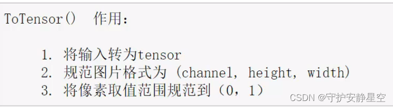
1.将输入转为Tensor，
2.将图片格式转换为通道在前，常见通道为（高，宽，通道（像素点rgb））转换为（通道（像素点rgb），高，宽）
3.将像素取值归一化
'''
minidat = torchvision.datasets.MNIST('data',#文件夹名字
									 train=True,#训练数据和测试数据选择
									 transform=ToTensor(),#转换方法
									 download=True)#第一次需要下载库
print(minidat)
s = DataLoader(minidat,batch_size=10)
print(s)
# print(x,y)
for x,y in s:
	print(x.shape,y.shape)
	torch.tensor()
'''
Dataset MNIST
    Number of datapoints: 60000
    Root location: data
    Split: Train
    StandardTransform
Transform: ToTensor()
<torch.utils.data.dataloader.DataLoader object at 0x00000254130BAC10>
tensor([[[[0., 0., 0.,  ..., 0., 0., 0.],
          [0., 0., 0.,  ..., 0., 0., 0.],
          [0., 0., 0.,  ..., 0., 0., 0.],
          ...,
          [0., 0., 0.,  ..., 0., 0., 0.],
          [0., 0., 0.,  ..., 0., 0., 0.],
          [0., 0., 0.,  ..., 0., 0., 0.]]],


        [[[0., 0., 0.,  ..., 0., 0., 0.],
          [0., 0., 0.,  ..., 0., 0., 0.],
          [0., 0., 0.,  ..., 0., 0., 0.],
          ...,
          [0., 0., 0.,  ..., 0., 0., 0.],
          [0., 0., 0.,  ..., 0., 0., 0.],
          [0., 0., 0.,  ..., 0., 0., 0.]]],


        [[[0., 0., 0.,  ..., 0., 0., 0.],
          [0., 0., 0.,  ..., 0., 0., 0.],
          [0., 0., 0.,  ..., 0., 0., 0.],
          ...,
          [0., 0., 0.,  ..., 0., 0., 0.],
          [0., 0., 0.,  ..., 0., 0., 0.],
          [0., 0., 0.,  ..., 0., 0., 0.]]],


        ...,


        [[[0., 0., 0.,  ..., 0., 0., 0.],
          [0., 0., 0.,  ..., 0., 0., 0.],
          [0., 0., 0.,  ..., 0., 0., 0.],
          ...,
          [0., 0., 0.,  ..., 0., 0., 0.],
          [0., 0., 0.,  ..., 0., 0., 0.],
          [0., 0., 0.,  ..., 0., 0., 0.]]],


        [[[0., 0., 0.,  ..., 0., 0., 0.],
          [0., 0., 0.,  ..., 0., 0., 0.],
          [0., 0., 0.,  ..., 0., 0., 0.],
          ...,
          [0., 0., 0.,  ..., 0., 0., 0.],
          [0., 0., 0.,  ..., 0., 0., 0.],
          [0., 0., 0.,  ..., 0., 0., 0.]]],


        [[[0., 0., 0.,  ..., 0., 0., 0.],
          [0., 0., 0.,  ..., 0., 0., 0.],
          [0., 0., 0.,  ..., 0., 0., 0.],
          ...,
          [0., 0., 0.,  ..., 0., 0., 0.],
          [0., 0., 0.,  ..., 0., 0., 0.],
          [0., 0., 0.,  ..., 0., 0., 0.]]]]) torch.Size([10])
'''

3.模型定义示例

这里举例定义一个简单的线性模型：


class model(nn.Module):
    def __init__(self):
        super().__init__()
        self.L1 = nn.Linear(28*28,1024)
        self.L2 = nn.Linear(1024,256)
        self.L3 = nn.Linear(256,10)
        self.leakRelu = nn.LeakyReLU()

    def forward(self,input):
        x = input.view(-1,28*28)
        x = self.L1(x)
        x = self.leakRelu(x)
        x = self.L2(x)
        x = self.leakRelu(x)
        logist = self.L3(x)
        return logist #一般没有经过激活的返回取名logist

4.模型训练

数据集固定方式之后，模型训练可以写一个固定的模型训练函数：

'''
m :模型
dl：训练数据集
optfun：优化函数
bach：全部数据训练批次
'''
def train(m,dl,lossfun,optfun,bach):
    # m = model()
    # dl = torch.utils.data.DataLoader()
    # lossfun = nn.CrossEntropyLoss
    # optfun = torch.optim.SGD()

    m.train()
    for count in np.arange(bach):
        for x,y in dl:
            y_pred = m(x)
            loss = lossfun(y_pred,y)
            optfun.zero_grad()
            loss.backward()
            optfun.step()
            with torch.no_grad():
                a = y_pred.argmax(1).data.numpy()
                b = y.data.numpy()
                c=((a==b).astype(np.int32).sum()/len(b))
                print('Prediction accuracy: ',c)
        print("Training times:",count)

5.模型存储与装载

在模型训练好以后可以存储起来代码：

'''
保存模型
 m 是模型
 p 是存储的文件名和路径
'''
def SaveModel(m,p):
    torch.save(m.state_dict(),p)

'''
装载模型
 p 是存储的文件名和路径
'''
def LoadModel(p):
    m = model()
    m.load_state_dict(torch.load(p))
    m.eval()
    return m

6.总结

对于 torchvision.transforms提供的转换工具函数使用示例：

#该方法把图像数据转化为tensor数据
trans_img = torchvision.transforms.ToTensor()
#转化方法如下
img = trans_img(img)

'''
如果一次要进行好几个转换可以合并转换功能
'''
trans_img = torchvision.transforms.Compose([torchvision.transforms.ToTensor(),
                                torchvision.transforms.ToPILImage()])
img = trans_img(img)

模型训练，保存，运用示例：

trans = torchvision.transforms.Compose([torchvision.transforms.ToTensor()])
    train_ds = torchvision.datasets.FashionMNIST('data',
                                          train=True,
                                          transform=trans,
                                          download=True)
    train_dl = DataLoader(train_ds,batch_size=128)
    test_ds = torchvision.datasets.FashionMNIST('data',
                                          train=True,
                                          transform=trans,
                                          download=False)
    test_dl = DataLoader(test_ds, batch_size=1)

    trans_img = torchvision.transforms.ToTensor()
    m_path = 'Fashion.pth'
    mod = model()
    lossfun = nn.CrossEntropyLoss()
    optfun = torch.optim.SGD(mod.parameters(),lr=0.001)

    # train(mod,train_dl,lossfun,optfun,100)
    # SaveModel(mod,m_path)

    mod = LoadModel(m_path)

    errCount = 0
    correctCount = 0
    for x,y in test_dl:
        y_pred=mod(x)

        print(y_pred.argmax(1),y)
        # cv.imshow(np.squeeze(x.data.numpy()))
        dy = y_pred.argmax(1)
        if dy.item()==y.item():
            correctCount+=1
        else:
            errCount+=1
    print('err:',errCount,'correct:',correctCount,correctCount/(correctCount+errCount))

后续关于继承Dataset，进行数据加载，会继续添加相关示例。