【机器学习】SVM（支持向量机）算法实验

(一)实验名称：SVM(支持向量机)算法实验

(二)实验目的：

1. 学习支持向量机SVM的基本概念
2. 了解核函数的基本概念
3. 掌握使用scikit-learn API函数实现SVM算法

(三)实验内容：使用scikit-learn API中的SVM算法解决非线性分类的问题

(四)实验原理

(五)实验步骤

1. 建立工程
2. 数据准备、分析
3. 模型训练
4. 模型可视化
5. 模型预测

相关代码如下

import numpy as np
import matplotlib.pyplot as plt
from sklearn.datasets import make_moons
from sklearn.preprocessing import PolynomialFeatures
from sklearn.preprocessing import StandardScaler
from sklearn.svm import LinearSVC
from sklearn.pipeline import Pipeline

import warnings
warnings.filterwarnings('ignore')

X,y=make_moons(n_samples=100,noise=0.1,random_state=1)
moonAxe=[-1.5,2.5,-1,1.5]

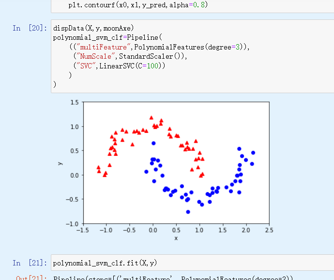
def dispData(x,y,moonAxe):
    pos_x0=[x[i,0] for i in range(len(y)) if y[i]==1]
    pos_x1=[x[i,1] for i in range(len(y)) if y[i]==1]
    neg_x0=[x[i,0] for i in range(len(y)) if y[i]==0]
    neg_x1=[x[i,1] for i in range(len(y)) if y[i]==0]
    
    plt.plot(pos_x0,pos_x1,"bo")
    plt.plot(neg_x0,neg_x1,"r^")        
            
    plt.axis(moonAxe)
    plt.xlabel("x")
    plt.ylabel("y")            

def disPredict(clf,moonAxe):
    d0=np.linspace(moonAxe[0],moonAxe[1],200)
    d1=np.linspace(moonAxe[2],moonAxe[3],200)
    x0,x1=np.meshgrid(d0,d1)
    X=np.c_[x0.ravel(),x1.ravel()]
    y_pred=clf.predict(X).reshape(x0.shape)
    plt.contourf(x0,x1,y_pred,alpha=0.8)

dispData(X,y,moonAxe)
polynomial_svm_clf=Pipeline(
    (("multiFeature",PolynomialFeatures(degree=3)),
     ("NumScale",StandardScaler()),
     ("SVC",LinearSVC(C=100))    
    )
)

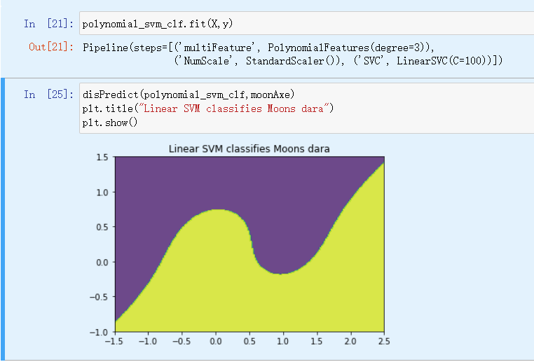
polynomial_svm_clf.fit(X,y)

disPredict(polynomial_svm_clf,moonAxe)
plt.title("Linear SVM classifies Moons dara")
plt.show()

相关结果的截图

写注释的代码

import numpy as np
import matplotlib.pyplot as plt
from sklearn.datasets import make_moons
from sklearn.preprocessing import PolynomialFeatures
from sklearn.preprocessing import StandardScaler
from sklearn.svm import LinearSVC
from sklearn.pipeline import Pipeline

import warnings
warnings.filterwarnings('ignore') # 忽略警告

# 生成半环形数据
X,y=make_moons(n_samples=100,noise=0.1,random_state=1)
moonAxe=[-1.5,2.5,-1,1.5] # moons数据集区间

# 显示数据样本
def dispData(x,y,moonAxe):
    pos_x0=[x[i,0] for i in range(len(y)) if y[i]==1]
    pos_x1=[x[i,1] for i in range(len(y)) if y[i]==1]
    neg_x0=[x[i,0] for i in range(len(y)) if y[i]==0]
    neg_x1=[x[i,1] for i in range(len(y)) if y[i]==0]
    
    plt.plot(pos_x0,pos_x1,"bo")
    plt.plot(neg_x0,neg_x1,"r^")        
            
    plt.axis(moonAxe)
    plt.xlabel("x")
    plt.ylabel("y")            

# 显示决策线
def disPredict(clf,moonAxe):
    # 生成区间内的数据
    d0=np.linspace(moonAxe[0],moonAxe[1],200)
    d1=np.linspace(moonAxe[2],moonAxe[3],200)
    x0,x1=np.meshgrid(d0,d1)
    X=np.c_[x0.ravel(),x1.ravel()]
    # 进行预测并绘制预测结果
    y_pred=clf.predict(X).reshape(x0.shape)
    plt.contourf(x0,x1,y_pred,alpha=0.8)

# 1.显示样本
dispData(X,y,moonAxe)
# 2.构建模型组合，整个三个函数
polynomial_svm_clf=Pipeline(
    (("multiFeature",PolynomialFeatures(degree=3)),
     ("NumScale",StandardScaler()),
     ("SVC",LinearSVC(C=100))    
    )
)

# 3.使用模块组合进行训练
polynomial_svm_clf.fit(X,y)

# 4.显示分类线
disPredict(polynomial_svm_clf,moonAxe)
# 5.设置图标标题
plt.title("Linear SVM classifies Moons dara")
plt.show()