渐进插值的LOOP 曲面细分

本文的算法来源于

哈尔滨理工大学孙立镌，鞠志涛的论文——渐进插值的LOOP 曲面细分

摘要

目前很多细分方法都存在不能用同一种方法处理封闭网格和开放网格的问题。对此，一种新的基于插值技术的LOOP 曲面细分方法，其主要思想就是给定一个初始三角网格$M$，反复生成新的顶点，新顶点是通过其相邻顶点的约束求解得到的，从而构造一个新的控制网格$\bar{M}$，在取极限的情况下，可以证明插值过程是收敛的;因为生成新顶点使用的是与其相连顶点的约束求解得到的，本质上是一种局部方法，所以，该方法很容易定义。它在本地方法和全局方法中都有优势，能处理任意顶点数量和任意拓扑结构的网格，从而产生一个光滑的曲面并忠实于给定曲面的形状，其控制网格可以是封闭的或者开放的。我们这里主要讨论的是封闭网格

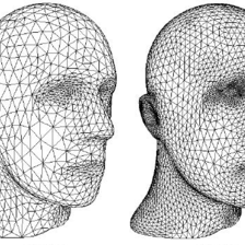
插值细分的几何细分过程

基于渐进插值的LOOP 曲面细分在封闭网格情况下的概念如下: 给定一个三维三角网格$M = M^0$ ，如果初始网格不是三
角网格要首先用Delaunay 三角化算法对网格进行处理。对LOOP 细分曲面的$M^0$插入新顶点，首先要找到一个封闭控制网格$\bar{M}$，使其LOOP 曲面通过$M^0$ 的所有顶点，其次要找到$\bar{M}$的顶点和$M^0$的顶点的直接关系。本文使用迭代的过程来进行这项工作。
考虑$M^0$ 上的LOOP 曲面$S^0$，对于$M^0$ 的每个顶点$V^0$，计算该顶点与它在$S^0$上的极限顶点$V^0_\infty$的距离为$D^0 =V^0-V^0_\infty$。将该距离与$V^0$相加得到细分一次后的顶点为$V^1= V^0 + D^0$。
所有顶点$V^1$的集合构成一次细分网格$M^1$，接下来计算$S^1$上的极限顶点$V^1_\infty$与$V^0$的距离为$D^1=V^0-V^1_\infty$。将该距离与$V^1$相加得到细分一次后的顶点为$V^2= V^1 + D^1$。
所有$V^2$构成第二次细分网格$M^2$ ，重复该过程可以得到第$k$次插值后的控制网格$M^k$，并且$D^k = V^0 － V^k_\infty$。
将这个距离与$V^k$相加得到$V^{k + 1}$为$V^{k + 1} = V^k + D^k$。所有
$V^{k + 1}$的集合构成$M^{k + 1}$。
这个过程产生了一系列控制网格$M^k$和一系列对应LOOP曲面$S^k$，如果当k 趋近于无穷时，$M^k$和$S^k$的距离趋近于0，就能证明该插值过程是收敛的，即$S^k$ 收敛于$M^0$。接下来就证明这
个结论。
注意到上述迭代过程的主要工作是计算$V^k\infty$，$V^k_\infty$是$S^k$上$V^k$对应的极限顶点。对于LOOP 曲面，通过价为n 的极限控制顶点的约束求解计算，约束方程如下:

$$\begin{gather} V_\infty=\beta_nV+(1-\beta_n)Q\ \ \ \ (1)\\ \beta_n=\frac{3}{11-8\times(\frac{3}{8}+(\frac{3}{8}+\frac{1}{4}\cos\frac{\pi}{n})^2)} (2)\\ Q=\frac{1}{n}\sum_{i=1}^nQ_i\ \ \ \ (3) \end{gather}$$
联立约束方程式(1) (2) (3) 可以求出 $V^k_{\infty}$，其中的 $Q_i$是V的邻域顶点。由于该计算过程只涉及V 的邻域顶点，该过程是一个局部方法，任何拓扑结构都可以利用该方法，即可以处理任意拓扑结构的网格。这里需要指出的是不必严格地一直按迭代过程计算下去，当 $M^0$ 和 $S^k$的距离小于给定的一个值时，就可以认为迭代过程已经符合要求。

程序实现及效果

程序实现

我修改了之前的loop细分程序，新的程序命名为adloopsub.m

function [newVertices, newFaces] =  adloopsub(vertices, faces)  
% Mesh subdivision using the Loop scheme.  
%  
%  Dimensions:  
%    vertices: 3xnVertices  
%    faces:    3xnFaces  
%    
%  Author: lafengxiaoyu 

    global edgeVertice;  
    global newIndexOfVertices;  
    newVertices = vertices;
    [originver, orifaces] = origin();

    nVertices = size(vertices,2);  
    nFaces    = size(faces,2);  
    edgeVertice = zeros(nVertices, nVertices, 3);  
    newDeff=vertices;
    newIndexOfVertices = nVertices;  

    % ------------------------------------------------------------------------ %  
    % create a matrix of edge-vertices and the new triangulation (newFaces).  
    % computational complexity = O(3*nFaces)  
    %   
    % * edgeVertice(x,y,1): index of the new vertice between (x,y)  
    % * edgeVertice(x,y,2): index of the first opposite vertex between (x,y)  
    % * edgeVertice(x,y,3): index of the second opposite vertex between (x,y)  
    %  
    %  0riginal vertices: va, vb, vc, vd.  
    %  New vertices: vp, vq, vr.  
    %  
    %      vb                   vb               
    %     / \                  /  \   
    %    /   \                vp--vq  
    %   /     \              / \  / \  
    % va ----- vc   ->     va-- vr --vc   
    %   \     /              \      /  
    %    \   /                \    /  
    %     \ /                  \  /  
    %      vd                   vd                 

    for i=1:nFaces  
        [vaIndex, vbIndex, vcIndex] = deal(faces(1,i), faces(2,i), faces(3,i));  

        addEdgeVertice(vaIndex, vbIndex, vcIndex);  
        addEdgeVertice(vbIndex, vcIndex, vaIndex);  
        addEdgeVertice(vaIndex, vcIndex, vbIndex);  

    end;  


    % ------------------------------------------------------------------------ %  
    % adjacent vertices (using edgeVertice)  
    adjVertice{nVertices} = [];  

    for v=1:nVertices  
        for vTmp=1:nVertices  
            if (v<vTmp && edgeVertice(v,vTmp,1)~=0) || (v>vTmp && edgeVertice(vTmp,v,1)~=0)  
                adjVertice{v}(end+1) = vTmp;  
            end;  
        end;      
    end;  

    % ------------------------------------------------------------------------ %  
    % new positions of the original vertices      
    for v=1:nVertices  
        k = length(adjVertice{v});  

        adjBoundaryVertices = [];  
        for i=1:k  
            vi = adjVertice{v}(i);  
            if (vi>v) && (edgeVertice(v,vi,3)==0) || (vi<v) && (edgeVertice(vi,v,3)==0)  
                adjBoundaryVertices(end+1) = vi;  
            end;  
        end;  

          beta = 3/(11-8*(3/8+((3/8 + 1/4*cos(2*pi/k))^2)));
          newVertices(:,v) = (beta)*vertices(:,v) + (1-beta)/k*sum(vertices(:,(adjVertice{v})),2);   
          newDeff(:,v)=originver(:,v)- newVertices(:,v);
          newVertices(:,v)=vertices(:,v)+newDeff(:,v);
    end;  
      newFaces=faces;
end  

% ---------------------------------------------------------------------------- %  
function vNIndex = addEdgeVertice(v1Index, v2Index, v3Index)  
    global edgeVertice;  
    global newIndexOfVertices;  

    if (v1Index>v2Index) % setting: v1 <= v2  
        vTmp = v1Index;  
        v1Index = v2Index;  
        v2Index = vTmp;  
    end;  

    if (edgeVertice(v1Index, v2Index, 1)==0)  % new vertex  
        newIndexOfVertices = newIndexOfVertices+1;  
        edgeVertice(v1Index, v2Index, 1) = newIndexOfVertices;  
        edgeVertice(v1Index, v2Index, 2) = v3Index;  
    else  
        edgeVertice(v1Index, v2Index, 3) = v3Index;  
    end;  

    vNIndex = edgeVertice(v1Index, v2Index, 1);  

    return;  
end  

其中origin.m用来读取数据

function [ vertices, faces ] = origin()
%ORIGIN 此处显示有关此函数的摘要
%   此处显示详细说明
%faces =load('C:\Users\Admin\Documents\MATLAB\face.txt');
%faces=faces+1;
%faces=faces';
%vertices =load('C:\Users\Admin\Documents\MATLAB\ver.txt');
%vertices=vertices';
[vertices, faces ]= obj__read( 'bunny_200.obj' );
%vertices=[-1 -1 0;-1 1 0;1 1 0]';
%faces=[1 2 3]';
end

效果

执行以下测试代码

[ vertices, faces ]=origin();
faces1=faces;vertices1=vertices;
%for i=1:5
%[vertices, faces] = adloopsub(vertices, faces);
%end

for i=1:3
[vertices, faces] = loopSubdivision(vertices, faces);
end

trimesh(faces', vertices(1,:), vertices(2,:), vertices(3,:),'LineWidth',1,'EdgeColor','k');alpha(0.0); hold on;
trimesh(faces1', vertices1(1,:), vertices1(2,:), vertices1(3,:),'EdgeColor','r');alpha(0.0);

obj_write('bunny1.obj',vertices,faces);

读入由200个点组成的兔子模型，分别进行loop细分和渐进loop细分，效果如下

loop细分三次后的兔子模型

渐进插值后loop三次的兔子模型

可以明显看得出来效果好一些

参考文献

［1］ LOOP C． Smooth subdivision surfaces based on triangles［D］． Utah:University of Utah，1987．
［2］ HALSTEAD M，KASS M，DEROSE T． Efficient，fair interpolation
using Catmull-Clark surfaces［C］/ /Proc of the 20th SIGGRAPH．1993: 47-61．
［3］ ZHENG Jian-min，CAI Y Yi-yu． Interpolation over arbitrary topology meshes using a two-phase subdivision scheme［J］． IEEE Trans on Visualization and Computer Graphics，2006，12( 3) : 301-310．
［4］ LAI Shu-hua，CHENG F． Similarity based interpolation using Catmull-Clark subdivision surfaces［J］． The Visual Computer，2006，22( 9) : 865-873．
［5］ ZORIN D，SCHRODER P，DEROSE T． Subdivision for modelingand animation［C］/ /Proc of SIGGRAPH． 2006: 30-50．
［6］ CHENG Fu-hua，FAN Feng-tao，LAI Shu-hua，et al． LOOP subdivision surface based progressive interpolation［J］． Journal of Computer Science and Technology，2009，24( 1) : 39-46．