通过Tensorflow和强化学习实现自动化吃豆人PacMan

　　介绍

　　在涉及GradientCrescent强化学习基础的文章中，我们研究了基于模型和基于样本的强化学习方法。 简而言之，前一类的特征是需要了解所有可能状态转换的完整概率分布，并且可以通过马尔可夫决策过程来举例说明。 相反，基于样本的学习方法只需要通过反复观察即可确定状态值，而无需进行转换动力学。 在这一领域中，我们涵盖了蒙特卡洛和时序差分学习。 简而言之，可以用状态值更新的频率将两者分开：虽然蒙特卡洛方法要求完成一集（episode）才能进行一轮更新，但时差方法使用状态的旧估计来增量更新内集值与折扣奖励一起生成新的更新。

　　时序差分学习（TD）或"在线"学习方法的快速反应性使其适合于高度动态的环境，因为状态和动作的值会通过估算集在整个时间内不断更新。 也许最值得注意的是，TD是Q-Leanring学习的基础，Q-Learning学习是一种更高级的算法，用于训练Agent应对诸如OpenAI Atari体育馆中观察到的游戏环境之类的游戏环境，也是本文的重点。

　　超越TD：SARSA和Q学习

　　回想一下在时序差分学习中，我们观察到一个主体通过状态（S），动作（A）和R（奖励Reward）的顺序在环境中循环地行为。

　　

　　由于这种周期性行为，我们可以在到达下一个状态后立即更新前一个状态的值。 但是，就像我们之前对马尔可夫决策过程所做的那样，我们可以将培训的范围扩展到包括状态-行动值。 这通常称为SARSA。 让我们比较状态动作和状态值TD更新方程：

　　

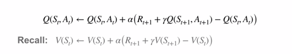
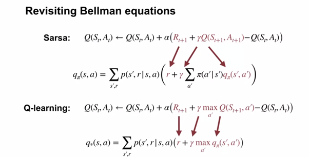
　　Q-learning学习通过在更新过程中强制选择具有最高动作值的动作来更进一步，这类似于使用Bellman最优性方程式观察到的方式。 我们可以在下面的Bellman和Bellman最优性方程式旁边检查SARSA和Q学习：

　　

　　考虑到需要不断地为现有动作值最高的状态选择动作，您可能想知道如何确保对状态动作空间的完整探索。 从理论上讲，我们可能因为不首先评估，就可以避开了最佳行动。 为了鼓励探索，我们可以使用递减的Epsilon greedy策略，从本质上讲，它迫使代理程序选择一个明显的次优操作，以便在一定百分比的时间内了解其价值。 通过引入衰减过程，我们可以在评估完所有状态后限制探索，然后我们将为每个状态永久选择最佳操作。

　　在我们之前使用基于MDP的模型处理Pong时，让我们了解一下有关Q学习的知识，并将其应用于Atari的《吃豆人》游戏。

　　实作

　　我们的Google Colaboratory实现是使用Tensorflow Core，用Python编写的，可以在GradientCrescent Github上找到。 它基于Ravichandiran等人的观点。 ，但已升级为与Tensorflow 2.0兼容，并进行了显著的扩展以促进更好的可视化和说明。 由于此方法的实现非常复杂，因此，我们总结一下所需的操作顺序：

　　我们定义了我们的深度Q-learning学习神经网络。 这是一个CNN，可获取游戏中的屏幕图像并输出Ms-Pacman游戏空间中每个动作或Q值的概率。 为了获得概率张量，我们在最后一层不包括任何激活函数。由于Q-learning学习需要我们了解当前状态和下一状态，因此我们需要从数据生成开始。 我们将代表初始状态s的游戏空间的预处理输入图像输入网络，并获取动作或Q值的初始概率分布。 在训练之前，这些值将显示为随机且次优。利用概率张量，然后使用argmax（）函数选择当前概率最高的操作，并使用它来构建epsilon贪婪策略。然后，根据我们的政策，我们选择动作a，并在gym环境中评估我们的决定，以接收有关新状态s，奖励r和情节是否结束的信息。我们将此信息组合以列表形式存储在缓冲区中，并重复步骤2-4进行预设次数，以建立足够大的缓冲区数据集。第5步完成后，我们开始生成损耗计算所需的目标y值R'和A'。 尽管前者只是从R打折而来，但我们通过将S'输入到我们的网络中来获得A'。有了所有组件之后，我们就可以计算损失来训练我们的网络。训练结束后，我们将以图形方式并通过演示评估代理的性能。

　　让我们开始吧。 随着Tensorflow 2在协作环境中的出现，我们已经使用新的compat软件包将代码转换为TF2兼容。 请注意，此代码不是TF2本机代码。

　　让我们导入所有必需的程序包，包括OpenAI gym 环境和Tensorflow核心。

　　import numpy as np

　　import gym

　　import tensorflow as tf

　　from tensorflow.contrib.layers import flatten, conv2d, fully_connected

　　from collections import deque, Counter

　　import random

　　from datetime import datetime

　　接下来，我们定义一个预处理功能，以从gym环境中裁剪图像并将其转换为一维张量。 我们在Pong自动化实施中已经看到了这一点。

　　def preprocess_observation(obs):

　　# Crop and resize the image

　　img=obs[1:176:2, ::2]

　　# Convert the image to greyscale

　　img=imgan(axis=2)

　　# Improve image contrast

　　img[img==color]=0

　　# Next we normalize the image from -1 to +1

　　img=(img — 128) / 128–1

　　return img.reshape(88,80,1)

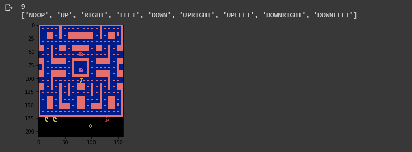
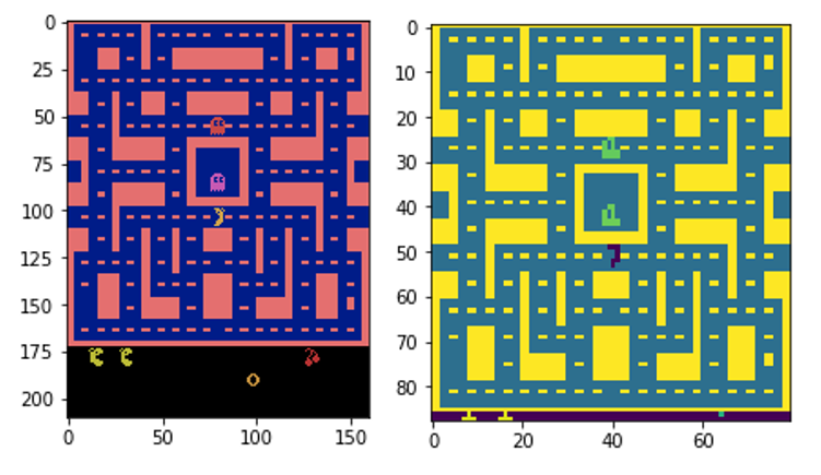
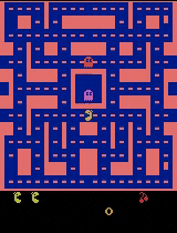
　　接下来，让我们初始化gym环境，检查几个游戏画面，并了解游戏空间中可用的9种动作。 当然，我们的代理无法获得此信息。

　　env=gym.make(“MsPacman-v0”)

　　n_outputs=env.action_space.n

　　print(n_outputs)

　　print(env.env.get_action_meanings())

　　observation=env.reset()

　　import tensorflow as tf

　　import matplotlib.pyplot as plt

　　for i in range(22):

　　if i > 20:

　　pltshow(observation)

　　plt()

　　observation, _, _, _=env.step(1)

　　您应注意以下几点：

　　

　　我们可以借此机会比较原始和预处理的输入图像：

　　

　　接下来，让我们定义我们的模型，即深度Q网络。 本质上，这是一个三层卷积网络，它获取预处理的输入图像，展平并将其馈送到完全连接的层，并输出在游戏空间中采取每个动作的概率。 如前所述，这里没有激活层，因为一个激活层会导致二进制输出分布。

　　def q_network(X, name_scope):

　　# Initialize layers

　　initializer=tfpat.v1.keras.initializers.VarianceScaling(scale=2.0)

　　with tfpat.v1.variable_scope(name_scope) as scope:

　　# initialize the convolutional layers

　　layer_1=conv2d(X, num_outputs=32, kernel_size=(8,8), stride=4, padding=’SAME’, weights_initializer=initializer)

　　tfpat.v1.summary.histogram(‘layer_1’,layer_1)

　　layer_2=conv2d(layer_1, num_outputs=64, kernel_size=(4,4), stride=2, padding=’SAME’, weights_initializer=initializer)

　　tfpat.v1.summary.histogram(‘layer_2’,layer_2)

　　layer_3=conv2d(layer_2, num_outputs=64, kernel_size=(3,3), stride=1, padding=’SAME’, weights_initializer=initializer)

　　tfpat.v1.summary.histogram(‘layer_3’,layer_3)

　　flat=flatten(layer_3)

　　fc=fully_connected(flat, num_outputs=128, weights_initializer=initializer)

　　tfpat.v1.summary.histogram(‘fc’,fc)

　　#Add final output layer

　　output=fully_connected(fc, num_outputs=n_outputs, activation_fn=None, weights_initializer=initializer)

　　tfpat.v1.summary.histogram(‘output’,output)

　　vars={v.name[len(scope.name):]: v for v in tfpat.v1.get_collection(key=tfpat.v1.GraphKeys.TRAINABLE_VARIABLES, scope=scope.name)}

　　#Return both variables and outputs together

　　return vars, output

　　让我们也借此机会为模型和训练过程定义我们的超参数

　　num_episodes=800

　　batch_size=48

　　input_shape=(None, 88, 80, 1)

　　#Recall shape is img.reshape(88,80,1)

　　learning_rate=0.001

　　X_shape=(None, 88, 80, 1)

　　discount_factor=0.97

　　global_step=0

　　copy_steps=100

　　steps_train=4

　　start_steps=2000

　　回想一下，Q学习要求我们选择具有最高动作值的动作。 为了确保我们仍然可以访问每个可能的状态行为组合，我们将让代理遵循epsilon-greedy政策，探索率为5％。 由于最终假设所有组合都已被探索，因此我们将设定此探索速率随时间衰减-在此之后的任何探索只会导致强制选择次优动作。

　　epsilon=0.5

　　eps_min=0.05

　　eps_max=1.0

　　eps_decay_steps=500000

　　#

　　def epsilon_greedy(action, step):

　　p=np.random.random(1).squeeze() #1D entries returned using squeeze

　　epsilon=max(eps_min, eps_max — (eps_max-eps_min) * step/eps_decay_steps) #Decaying policy with more steps

　　if np.random.rand() < epsilon:

　　return np.random.randint(n_outputs)

　　else:

　　return action

　　回想一下上面的公式，Q学习的更新功能需要满足以下条件：

　　当前状态当前动作当前动作后的奖励下一个状态下一个动作是

　　为了以有意义的数量提供这些参数，我们需要根据一组参数评估当前策略，并将所有变量存储在缓冲区中，在训练期间，我们将从这些缓冲区中提取数据。 在Pong，我们使用了增量方法。 让我们继续创建缓冲区和一个简单的采样函数：

　　buffer_len=20000

　　#Buffer is made from a deque — double ended queue

　　exp_buffer=deque(maxlen=buffer_len)

　　def sample_memories(batch_size):

　　perm_batch=np.random.permutation(len(exp_buffer))[:batch_size]

　　mem=np.array(exp_buffer)[perm_batch]

　　return mem[:,0], mem[:,1], mem[:,2], mem[:,3], mem[:,4]

　　接下来，让我们将原始网络的权重参数复制到目标网络中。 这种双网络方法使我们可以在训练过程中使用现有策略生成数据，同时仍为下一次策略迭代优化参数。

　　# we build our Q network, which takes the input X and generates Q values for all the actions in the state

　　mainQ, mainQ_outputs=q_network(X, ‘mainQ’)

　　# similarly we build our target Q network, for policy evaluation

　　targetQ, targetQ_outputs=q_network(X, ‘targetQ’)

　　copy_op=[tfpat.v1.assign(main_name, targetQ[var_name]) for var_name, main_name in mainQ.items()]

　　copy_target_to_main=tf(*copy_op)

　　最后，我们还要定义损失。 这只是我们的目标操作（具有最高操作值）和我们的预测操作的平方差。 我们将使用ADAM优化器来最大程度地减少训练过程中的损失。

　　# define a placeholder for our output i.e action

　　y=tfpat.v1.placeholder(tf.float32, shape=(None,1))

　　# now we calculate the loss which is the difference between actual value and predicted value

　　loss=tfuce_mean(input_tensor=tf.square(y — Q_action))

　　# we use adam optimizer for minimizing the loss

　　optimizer=tfpat.v1.train.AdamOptimizer(learning_rate)

　　training_op=optimizer.minimize(loss)

　　init=tfpat.v1.global_variables_initializer()

　　loss_summary=tfpat.v1.summary.scalar(‘LOSS’, loss)

　　merge_summary=tfpat.v1.summaryrge_all()

　　file_writer=tfpat.v1.summary.FileWriter(logdir, tfpat.v1.get_default_graph())

　　定义好所有代码后，我们就可以运行我们的网络并完成训练过程。 我们在初始摘要中已定义了大部分内容，但让我们回顾一下后代。

　　对于每个epoch，在使用epsilon-greedy策略选择下一个动作之前，我们将输入图像馈入网络以生成可用动作的概率分布。然后，我们将其输入到gym环境中，并获取有关下一个状态和伴随奖励的信息，并将其存储在我们的缓冲区中。在缓冲区足够大之后，我们将下一个状态采样到我们的网络中以获得下一个动作。 我们还通过折现当前奖励来计算下一个奖励我们通过Q-learning学习更新功能生成目标y值，并训练我们的网络。通过最大程度地减少训练损失，我们更新了网络权重参数，以便为下一个策略输出改进的状态操作值。

　　with tfpat.v1.Session() as sess:

　　init()

　　# for each episode

　　history=[]

　　for i in range(num_episodes):

　　done=False

　　obs=env.reset()

　　epoch=0

　　episodic_reward=0

　　actions_counter=Counter()

　　episodic_loss=[]

　　# while the state is not the terminal state

　　while not done:

　　# get the preprocessed game screen

　　obs=preprocess_observation(obs)

　　# feed the game screen and get the Q values for each action,

　　actions=mainQ_outputs.eval(feed_dict={X:[obs], in_training_mode:False})

　　# get the action

　　action=np.argmax(actions, axis=-1)

　　actions_counter[str(action)] +=1

　　# select the action using epsilon greedy policy

　　action=epsilon_greedy(action, global_step)

　　# now perform the action and move to the next state, next_obs, receive reward

　　next_obs, reward, done, _=env.step(action)

　　# Store this transition as an experience in the replay buffer! Quite important

　　exp_buffer.append([obs, action, preprocess_observation(next_obs), reward, done])

　　# After certain steps we move on to generating y-values for Q network with samples from the experience replay buffer

　　if global_step % steps_train==0 and global_step > start_steps:

　　o_obs, o_act, o_next_obs, o_rew, o_done=sample_memories(batch_size)

　　# states

　　o_obs=[x for x in o_obs]

　　# next states

　　o_next_obs=[x for x in o_next_obs]

　　# next actions

　　next_act=mainQ_outputs.eval(feed_dict={X:o_next_obs, in_training_mode:False})

　　#discounted reward for action: these are our Y-values

　　y_batch=o_rew + discount_factor * np.max(next_act, axis=-1) * (1-o_done)

　　# merge all summaries and write to the file

　　mrg_summary=merge_summary.eval(feed_dict={X:o_obs, y:np.expand_dims(y_batch, axis=-1), X_action:o_act, in_training_mode:False})

　　file_writer.add_summary(mrg_summary, global_step)

　　# To calculate the loss, we run the previously defined functions mentioned while feeding inputs

　　train_loss, _=sess([loss, training_op], feed_dict={X:o_obs, y:np.expand_dims(y_batch, axis=-1), X_action:o_act, in_training_mode:True})

　　episodic_loss.append(train_loss)

　　# after some interval we copy our main Q network weights to target Q network

　　if (global_step+1) % copy_steps==0 and global_step > start_steps:

　　copy_target_to_main()

　　obs=next_obs

　　epoch +=1

　　global_step +=1

　　episodic_reward +=reward

　　history.append(episodic_reward)

　　print(‘Epochs per episode:’, epoch, ‘Episode Reward:’, episodic_reward,”Episode number:”, len(history))

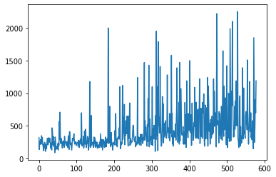
　　训练完成后，我们可以针对增量情节绘制奖励分布。 前550集（大约2小时）如下所示：

　　

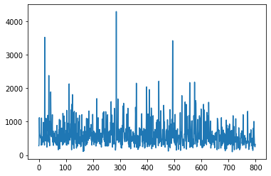
　　再过800集后，这会收敛到以下内容：

　　

　　为了在协作环境的限制内评估结果，我们可以记录整个情节并使用基于IPython库的包装在虚拟显示器中显示它：

　　'''Utility functions to enable video recording of gym environment and displaying it. To enable video, just do “env=wrap_env(env)"'''

　　def show_video():

　　mp4list=glob.glob(‘video/*.mp4’)

　　if len(mp4list) > 0:

　　mp4=mp4list[0]

　　video=io.open(mp4, ‘r+b’).read()

　　encoded=base64.b64encode(video)

　　ipythondisplay.display(HTML(data=’’’

　　loop controls style=”height: 400px;”>

　　

　　’’’.format(encoded.decode(‘ascii’))))

　　else:

　　print(“Could not find video”)

　　def wrap_env(env):

　　env=Monitor(env, ‘./video’, force=True)

　　return env

　　然后，我们使用模型运行环境的新会话并进行记录。

　　#Evaluate model on openAi GYM

　　observation=env.reset()

　　new_observation=observation

　　prev_input=None

　　done=False

　　with tfpat.v1.Session() as sess:

　　init()

　　while True:

　　if True:

　　#set input to network to be difference image

　　obs=preprocess_observation(observation)

　　# feed the game screen and get the Q values for each action

　　actions=mainQ_outputs.eval(feed_dict={X:[obs], in_training_mode:False})

　　# get the action

　　action=np.argmax(actions, axis=-1)

　　actions_counter[str(action)] +=1

　　# select the action using epsilon greedy policy

　　action=epsilon_greedy(action, global_step)

　　envder()

　　observation=new_observation

　　# now perform the action and move to the next state, next_obs, receive reward

　　new_observation, reward, done, _=env.step(action)

　　if done:

　　#observation=env.reset()

　　break

　　env.close()

　　show_video()

　　您应该观察游戏的一些回合！ 这是我们录制的几集。

　　

　　

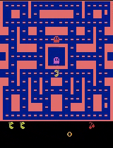
　　对于经过数小时训练的模型来说，还不错，得分超过400。特别是，当我们的代理直接被幽灵追赶时，它的表现似乎不错，但在预测来袭者方面仍然表现欠佳，可能是因为它没有足够的经验来观察他们的动作呢。

　　到此结束了对Q-learning学习的介绍。 在我们的下一篇文章中，我们将从Atari的世界转向解决世界上最著名的FPS游戏之一。 敬请关注！

　　参考文献

　　Sutton et. al，强化学习White et. al，艾伯塔大学强化学习基础Silva et. al，强化学习，UCLRavichandiran et. al，使用Python进行动手强化学习