%% 初始设置
clear; clc; close all;
rng(0); % 设置随机种子以保证结果可重现
warning(‘off’, ‘all’); % 关闭所有警告
% 设置全局字体为Times New Roman
set(0, ‘DefaultAxesFontName’, ‘Times New Roman’);
set(0, ‘DefaultTextFontName’, ‘Times New Roman’);
set(0, ‘DefaultLegendFontName’, ‘Times New Roman’);
set(0, ‘DefaultColorbarFontName’, ‘Times New Roman’);
%% 1. 从Excel文件读取数据
% 指定Excel文件路径
excel_file = “C:\Users\汤伟娟\Desktop\data.xlsx”; % 修改为实际路径
% 读取数据
data = xlsread(excel_file);
% 移除包含NaN的行
valid_rows = ~any(isnan(data(:,2:3)), 2);
data = data(valid_rows, 😃;
years = data(:,1); % 第一列:年份
x1 = data(:,2); % 第二列:风速
x2 = data(:,3); % 第三列:温度(含负值)
% 显示数据基本信息
fprintf(‘数据读取完成,共 %d 条记录\n’, length(x1));
fprintf(‘风速范围: %.2f 到 %.2f m/s\n’, min(x1), max(x1));
fprintf(‘温度范围: %.2f 到 %.2f °C\n’, min(x2), max(x2));
%% 2. 计算Kendall tau相关系数
n = length(x1);
tau = corr(x1, x2, ‘type’, ‘Kendall’);
fprintf(‘Kendall tau 相关系数: %.4f\n’, tau);
%% 3. 边缘分布拟合
% 风速边缘分布 - 使用广义极值分布 (GEV)
fprintf(‘\n===== 风速边缘分布 =====\n’);
fprintf(‘分布类型: 广义极值分布 (GEV)\n’);
% 拟合GEV分布
pd1 = fitdist(x1, ‘GeneralizedExtremeValue’);
y_cdf1 = cdf(pd1, x1);
fprintf(‘参数: k = %.4f, sigma = %.4f, mu = %.4f\n’, pd1.k, pd1.sigma, pd1.mu);
% 温度边缘分布 - 使用混合高斯分布 (GMM)
fprintf(‘\n===== 温度边缘分布拟合 (混合高斯分布) =====\n’);
% 确定最佳混合分量数 (1-5)
best_bic = Inf; % 使用BIC代替AIC
best_gmm = [];
best_k = 1;
for k = 1:5
try
options = statset(‘MaxIter’, 1000, ‘TolFun’, 1e-6);
gmm = fitgmdist(x2, k, ‘Options’, options, ‘Replicates’, 5);
% 手动计算BIC logL = gmm.NegativeLogLikelihood * -1; % 获取正对数似然 numParams = 3*k - 1; % 参数数量: k个均值 + k个方差 + (k-1)个混合比例 bic_val = -2*logL + numParams*log(n); fprintf('分量数: %d, BIC: %.4f\n', k, bic_val); if bic_val < best_bic best_bic = bic_val; best_gmm = gmm; best_k = k; end catch ME fprintf('分量数 %d 拟合失败: %s\n', k, ME.message); end
end
if isempty(best_gmm)
error(‘所有混合高斯分布拟合失败,请尝试其他分布类型’);
end
pd2 = best_gmm;
fprintf(‘\n最优混合高斯分布: %d 个分量, BIC = %.4f\n’, best_k, best_bic);
disp(pd2);
% 创建自定义CDF函数用于混合高斯分布
gmm_cdf = @(x) arrayfun(@(val) cdf(pd2, val), x);
% 计算温度CDF
y_cdf2 = gmm_cdf(x2);
% 绘制边缘分布拟合图
figure;
subplot(2,1,1);
hold on;
histogram(x1, 20, ‘Normalization’, ‘pdf’, ‘FaceColor’, [0.7 0.7 0.9]);
% 绘制GEV分布PDF
x_values_wind = linspace(min(x1), max(x1), 200)';
pdf_values_wind = pdf(pd1, x_values_wind);
plot(x_values_wind, pdf_values_wind, ‘r-’, ‘LineWidth’, 2);
title(‘风速分布拟合 (GEV)’, ‘FontName’, ‘Times New Roman’);
xlabel(‘风速 (m/s)’, ‘FontName’, ‘Times New Roman’);
ylabel(‘概率密度’, ‘FontName’, ‘Times New Roman’);
legend(‘数据’, ‘GEV拟合’, ‘Location’, ‘best’, ‘FontName’, ‘Times New Roman’);
grid on;
set(gca, ‘FontName’, ‘Times New Roman’);
subplot(2,1,2);
hold on;
histogram(x2, 20, ‘Normalization’, ‘pdf’, ‘FaceColor’, [0.7 0.7 0.9]);
% 绘制混合高斯分布PDF
x_values_temp = linspace(min(x2), max(x2), 200)'; % 转换为列向量
pdf_values_temp = pdf(pd2, x_values_temp);
plot(x_values_temp, pdf_values_temp, ‘r-’, ‘LineWidth’, 2);
% 绘制各分量PDF
if best_k > 1
colors = lines(best_k);
for m = 1:best_k
mu = pd2.mu(m);
sigma = sqrt(pd2.Sigma(1,1,m)); % 修正协方差索引
weight = pd2.ComponentProportion(m);
comp_pdf = weight * normpdf(x_values_temp, mu, sigma);
plot(x_values_temp, comp_pdf, ‘–’, ‘Color’, colors(m,:), ‘LineWidth’, 1);
end
end
title(sprintf(‘温度分布拟合 (混合高斯分布, %d个分量)’, best_k), ‘FontName’, ‘Times New Roman’);
xlabel(‘温度 (°C)’, ‘FontName’, ‘Times New Roman’);
ylabel(‘概率密度’, ‘FontName’, ‘Times New Roman’);
if best_k > 1
legend_txt = cell(1, best_k+1);
legend_txt{1} = ‘数据’;
legend_txt{2} = ‘混合PDF’;
for m = 1:best_k
legend_txt{m+2} = sprintf(‘分量%d’, m);
end
legend(legend_txt, ‘Location’, ‘best’, ‘FontName’, ‘Times New Roman’);
else
legend(‘数据’, ‘拟合曲线’, ‘FontName’, ‘Times New Roman’);
end
grid on;
set(gca, ‘FontName’, ‘Times New Roman’);
U = y_cdf1;
V = y_cdf2;
% 确保U和V在(0,1)范围内 (修复边界问题)
eps = 1e-5;
U = min(max(U, eps), 1-eps);
V = min(max(V, eps), 1-eps);
%% 4. Copula参数估计
fprintf(‘\n===== Copula参数估计 =====\n’);
% Gaussian Copula
rho_Gaussian = copulafit(‘Gaussian’, [U(😃, V(😃]);
fprintf(‘Gaussian Copula 参数: rho = %.4f\n’, rho_Gaussian);
% t-Copula
[rho_t, nuhat] = copulafit(‘t’, [U(😃, V(😃]);
fprintf(‘t-Copula 参数: rho = %.4f, nu = %.4f\n’, rho_t, nuhat);
% Frank Copula
rho_Frank = copulafit(‘Frank’, [U(😃, V(😃]);
fprintf(‘Frank Copula 参数: alpha = %.4f\n’, rho_Frank);
% Gumbel Copula
rho_Gumbel = copulafit(‘Gumbel’, [U(😃, V(😃]);
fprintf(‘Gumbel Copula 参数: alpha = %.4f\n’, rho_Gumbel);
% Clayton Copula
rho_Clayton = copulafit(‘Clayton’, [U(😃, V(😃]);
fprintf(‘Clayton Copula 参数: alpha = %.4f\n’, rho_Clayton);
%% 5. 计算5种copula的BIC值
parameter_Gaussian = 1;
CDF_Gaussian = copulacdf(‘Gaussian’, [U(😃, V(😃], rho_Gaussian);
BIC_gaussian = -2*sum(log(CDF_Gaussian)) + log(n)*parameter_Gaussian;
parameter_t = 2;
CDF_t = copulacdf(‘t’, [U(😃, V(😃], rho_t, nuhat);
BIC_t = -2*sum(log(CDF_t)) + log(n)*parameter_t;
parameter_Frank = 1;
CDF_Frank = copulacdf(‘Frank’, [U(😃, V(😃], rho_Frank);
BIC_Frank = -2*sum(log(CDF_Frank)) + log(n)*parameter_Frank;
parameter_Gumbel = 1;
CDF_Gumbel = copulacdf(‘Gumbel’, [U(😃, V(😃], rho_Gumbel);
BIC_Gumbel = -2*sum(log(CDF_Gumbel)) + log(n)*parameter_Gumbel;
parameter_Clayton = 1;
CDF_Clayton = copulacdf(‘Clayton’, [U(😃, V(😃], rho_Clayton);
BIC_Clayton = -2*sum(log(CDF_Clayton)) + log(n)*parameter_Clayton;
% 显示BIC值
fprintf(‘\n===== Copula BIC值 =====\n’);
fprintf(‘Gaussian: %.4f\n’, BIC_gaussian);
fprintf(‘t: %.4f\n’, BIC_t);
fprintf(‘Frank: %.4f\n’, BIC_Frank);
fprintf(‘Gumbel: %.4f\n’, BIC_Gumbel);
fprintf(‘Clayton: %.4f\n’, BIC_Clayton);
%% 6. 计算经验Copula函数
[fx, xsort] = ecdf(x1);
[fx1, x1sort] = ecdf(x2);
U1 = spline(xsort(2:end), fx(2:end), x1);
V1 = spline(x1sort(2:end), fx1(2:end), x2);
% 定义经验Copula函数
C = @(u,v) mean((U1 <= u) & (V1 <= v));
CUV = arrayfun(@(i) C(U1(i), V1(i)), 1:numel(U))';
%% 7. 计算理论Copula函数值
C_Gaussian = copulacdf(‘Gaussian’, [U(😃, V(😃], rho_Gaussian);
C_t = copulacdf(‘t’, [U(😃, V(😃], rho_t, nuhat);
C_Frank = copulacdf(‘Frank’, [U(😃, V(😃], rho_Frank);
C_Gumbel = copulacdf(‘Gumbel’, [U(😃, V(😃], rho_Gumbel);
C_Clayton = copulacdf(‘Clayton’, [U(😃, V(😃], rho_Clayton);
%% 8. 计算平方欧氏距离和RMSE
d2_Gaussian = sum((CUV - C_Gaussian).^2);
d2_t = sum((CUV - C_t).^2);
d2_Frank = sum((CUV - C_Frank).^2);
d2_Gumbel = sum((CUV - C_Gumbel).^2);
d2_Clayton = sum((CUV - C_Clayton).^2);
RMSE_Gaussian = sqrt(d2_Gaussian/n);
RMSE_t = sqrt(d2_t/n);
RMSE_Frank = sqrt(d2_Frank/n);
RMSE_Gumbel = sqrt(d2_Gumbel/n);
RMSE_Clayton = sqrt(d2_Clayton/n);
% 显示RMSE值
fprintf(‘\n===== Copula RMSE值 =====\n’);
fprintf(‘Gaussian: %.6f\n’, RMSE_Gaussian);
fprintf(‘t: %.6f\n’, RMSE_t);
fprintf(‘Frank: %.6f\n’, RMSE_Frank);
fprintf(‘Gumbel: %.6f\n’, RMSE_Gumbel);
fprintf(‘Clayton: %.6f\n’, RMSE_Clayton);
%% 9. 选择最优Copula(基于BIC和RMSE)
BICs = [BIC_gaussian, BIC_t, BIC_Frank, BIC_Gumbel, BIC_Clayton];
RMSEs = [RMSE_Gaussian, RMSE_t, RMSE_Frank, RMSE_Gumbel, RMSE_Clayton];
copula_names = {‘Gaussian’, ‘t’, ‘Frank’, ‘Gumbel’, ‘Clayton’};
% 找到BIC最小和RMSE最小的Copula
[~, idx_bic] = min(BICs);
[~, idx_rmse] = min(RMSEs);
fprintf(‘\n===== Copula选择结果 =====\n’);
fprintf(‘最优Copula (BIC准则): %s (BIC=%.4f)\n’, copula_names{idx_bic}, BICs(idx_bic));
fprintf(‘最优Copula (RMSE准则): %s (RMSE=%.6f)\n’, copula_names{idx_rmse}, RMSEs(idx_rmse));
% 使用BIC准则选择的最优Copula
optimal_copula = copula_names{idx_bic};
switch optimal_copula
case ‘Gaussian’
rho = rho_Gaussian;
copula_fun = ‘Gaussian’;
case ‘t’
rho = rho_t;
nu = nuhat;
copula_fun = ‘t’;
case ‘Frank’
rho = rho_Frank;
copula_fun = ‘Frank’;
case ‘Gumbel’
rho = rho_Gumbel;
copula_fun = ‘Gumbel’;
case ‘Clayton’
rho = rho_Clayton;
copula_fun = ‘Clayton’;
end
%% 10. 基于Copula的联合分布计算
% 设置合理的网格范围(风速固定为0-12,温度固定为-16到-8)
wind_min = 0; % 风速最小值固定为0
wind_max = 12; % 风速最大值固定为12
temp_min = -16; % 温度最小值固定为-16
temp_max = -8; % 温度最大值固定为-8
fprintf(‘\n网格范围设置:\n’);
fprintf(‘风速: %.2f 到 %.2f m/s\n’, wind_min, wind_max);
fprintf(‘温度: %.2f 到 %.2f °C\n’, temp_min, temp_max);
x11 = linspace(wind_min, wind_max, 100); % 风速网格 (0-12 m/s)
x22 = linspace(temp_min, temp_max, 100); % 温度网格(固定范围-16到-8°C)
% 初始化矩阵
ZZ = zeros(length(x22), length(x11)); % CDF
PP = zeros(length(x22), length(x11)); % PDF
RR = zeros(length(x22), length(x11)); % 联合重现期
Tongxian = zeros(length(x22), length(x11)); % 同现概率
Tongxian_RP = zeros(length(x22), length(x11)); % 同现重现期
fprintf(‘\n计算联合分布…\n’);
progress = 0;
total_iter = length(x11) * length(x22);
for i = 1:length(x11)
for j = 1:length(x22)
% 计算当前进度
current_iter = (i-1)length(x22) + j;
if mod(current_iter, 1000) == 0
fprintf(‘进度: %.1f%%\n’, 100current_iter/total_iter);
end
% 风速CDF - 使用GEV分布 u1 = cdf(pd1, x11(i)); % 温度CDF - 使用混合高斯分布的自定义CDF函数 u2 = gmm_cdf(x22(j)); % 避免边界问题 eps = 1e-5; u1 = min(max(u1, eps), 1-eps); u2 = min(max(u2, eps), 1-eps); % 应用最优Copula switch optimal_copula case 'Gaussian' C_val = copulacdf('Gaussian', [u1, u2], rho); P_val = copulapdf('Gaussian', [u1, u2], rho); case 't' C_val = copulacdf('t', [u1, u2], rho, nu); P_val = copulapdf('t', [u1, u2], rho, nu); case 'Frank' C_val = copulacdf('Frank', [u1, u2], rho); P_val = copulapdf('Frank', [u1, u2], rho); case 'Gumbel' C_val = copulacdf('Gumbel', [u1, u2], rho); P_val = copulapdf('Gumbel', [u1, u2], rho); case 'Clayton' C_val = copulacdf('Clayton', [u1, u2], rho); P_val = copulapdf('Clayton', [u1, u2], rho); end ZZ(j,i) = C_val; PP(j,i) = P_val; RR(j,i) = 1/(1 - C_val); % 联合重现期 Tongxian(j,i) = 1 - u1 - u2 + C_val; % 同现概率 Tongxian_RP(j,i) = 1/Tongxian(j,i); % 同现重现期 end
end
fprintf(‘联合分布计算完成!\n’);
[XX, YY] = meshgrid(x11, x22);
%% 11. 可视化结果
% 1. 二维联合概率分布图(CDF等值线图)
figure;
contourf(XX, YY, ZZ, 15, ‘ShowText’, ‘on’);
colorbar;
caxis([0 1]);
xlabel(‘风速 (m/s)’, ‘FontName’, ‘Times New Roman’);
ylabel(‘温度 (°C)’, ‘FontName’, ‘Times New Roman’);
title(‘’);
grid on;
ylim([-16, -8]); % 添加温度范围限制
set(gcf, ‘Position’, [100, 100, 800, 600]);
set(gca, ‘FontName’, ‘Times New Roman’);
saveas(gcf, ‘Joint_Probability_Distribution.png’);
% 2. 二维联合概率密度图(PDF等值线图)
figure;
contourf(XX, YY, PP, 15, ‘ShowText’, ‘on’);
colorbar;
xlabel(‘风速 (m/s)’, ‘FontName’, ‘Times New Roman’);
ylabel(‘温度 (°C)’, ‘FontName’, ‘Times New Roman’);
title(‘’);
grid on;
ylim([-16, -8]); % 添加温度范围限制
set(gcf, ‘Position’, [100, 100, 800, 600]);
set(gca, ‘FontName’, ‘Times New Roman’);
saveas(gcf, ‘Joint_Probability_Density.png’);
% 二维联合概率分布3D曲面图
figure;
surf(XX, YY, ZZ, ‘EdgeColor’, ‘none’, ‘FaceAlpha’, 0.8);
shading interp;
colormap(jet);
colorbar;
caxis([0 1]);
xlabel(‘风速 (m/s)’, ‘FontName’, ‘Times New Roman’);
ylabel(‘温度 (°C)’, ‘FontName’, ‘Times New Roman’);
zlabel(‘联合概率’, ‘FontName’, ‘Times New Roman’);
title(‘二维联合概率分布 (CDF 3D视图)’, ‘FontName’, ‘Times New Roman’);
view(30, 30);
grid on;
ylim([-16, -8]); % 添加温度范围限制
set(gca, ‘FontName’, ‘Times New Roman’);
saveas(gcf, ‘Joint_Probability_3D.png’);
%% 12. 优化二维联合概率分布3D曲面图
figure;
set(gcf, ‘Position’, [100, 100, 1000, 800], ‘Color’, ‘white’); % 设置背景为白色
% 创建3D曲面图
s = surf(XX, YY, ZZ, ‘EdgeColor’, ‘none’, ‘FaceAlpha’, 0.85);
shading interp;
% 设置颜色映射
colormap(parula); % 使用更科学的parula色彩方案
c = colorbar(‘Location’, ‘eastoutside’);
c.Label.String = ‘联合概率’;
c.Label.FontSize = 20;
c.Label.FontWeight = ‘bold’;
c.Label.FontName = ‘Times New Roman’;
caxis([0 1]);
set(c, ‘FontName’, ‘Times New Roman’);
% 设置坐标轴标签
xlabel(‘风速 (m/s)’, ‘FontSize’, 20, ‘FontWeight’, ‘bold’, ‘FontName’, ‘Times New Roman’);
ylabel(‘温度 (°C)’, ‘FontSize’, 20, ‘FontWeight’, ‘bold’, ‘FontName’, ‘Times New Roman’);
zlabel(‘联合概率’, ‘FontSize’, 20, ‘FontWeight’, ‘bold’, ‘FontName’, ‘Times New Roman’);
% 设置标题
title(‘’, ‘FontSize’, 16, ‘FontWeight’, ‘bold’, ‘FontName’, ‘Times New Roman’);
% 设置视角和光照
view(45, 35); % 调整到更优视角
light(‘Position’, [10 10 10], ‘Style’, ‘infinite’);
lighting gouraud; % 使用Gouraud光照模型
s.FaceLighting = ‘gouraud’;
s.AmbientStrength = 0.3;
s.DiffuseStrength = 0.8;
s.SpecularStrength = 0.1;
s.SpecularExponent = 25;
s.BackFaceLighting = ‘lit’;
% 设置坐标轴范围和网格
xlim([0 12]);
ylim([-16 -8]); % 确保温度范围在-16到-8
zlim([0 1]);
grid on;
set(gca, ‘FontSize’, 20, ‘LineWidth’, 1.5, ‘Box’, ‘on’, …
‘XMinorGrid’, ‘on’, ‘YMinorGrid’, ‘on’, ‘ZMinorGrid’, ‘on’, …
‘FontName’, ‘Times New Roman’);
% 设置背景和视角
set(gca, ‘Color’, [0.95 0.95 0.95]); % 浅灰色背景
set(gcf, ‘InvertHardcopy’, ‘off’); % 保持背景颜色
% 保存高质量图像
saveas(gcf, ‘Enhanced_Joint_Probability_3D.png’);
print(‘Enhanced_Joint_Probability_3D’, ‘-dpng’, ‘-r300’); % 300 DPI分辨率
% 设置默认字体大小
set(groot, ‘defaultAxesFontSize’, 20);
% 创建图形
figure;
scatter(CUV, C_Gaussian, 30, ‘filled’, ‘MarkerFaceAlpha’, 0.6);
hold on;
plot([0, 1], [0, 1], ‘r-’, ‘LineWidth’, 2);
% 使用更安全的标签设置方式
xlabel(‘经验Copula’, ‘FontName’, ‘Times New Roman’);
ylabel(‘Gumbel Copula’, ‘FontName’, ‘Times New Roman’);
title(‘’, ‘FontName’, ‘Times New Roman’);
% 图形设置
grid on;
axis equal;
xlim([0, 1]);
ylim([0, 1]);
set(gca, ‘FontName’, ‘Times New Roman’);
% 修正Position参数(注意逗号分隔)
set(gcf, ‘Position’, [100, 100, 800, 600]);
% 使用print保存高分辨率图像
print(gcf, ‘Empirical_vs_Theoretical_Copula.png’, ‘-dpng’, ‘-r300’);
%% 新增:三维联合概率密度图
% 计算网格上的边缘密度(修复维度问题)
f1_vals = pdf(pd1, x11); % 风速边缘密度 (1x100)
% 对于混合高斯分布,需要单独计算每个点的PDF
f2_vals = arrayfun(@(t) pdf(pd2, t), x22); % 温度边缘密度 (1x100)
% 创建边缘密度网格
[F1, F2] = meshgrid(f1_vals, f2_vals);
% 计算联合概率密度 = copula密度 × 边缘密度1 × 边缘密度2
Joint_Density = PP .* F1 .* F2;
% 绘制三维联合概率密度图
figure;
set(gcf, ‘Position’, [100, 100, 1000, 800], ‘Color’, ‘white’);
s = surf(XX, YY, Joint_Density, ‘EdgeColor’, ‘none’, ‘FaceAlpha’, 0.85);
shading interp;
% 设置颜色映射
colormap(parula);
c = colorbar(‘eastoutside’);
c.Label.String = ‘联合概率密度’;
c.Label.FontSize = 20;
c.Label.FontWeight = ‘bold’;
c.Label.FontName = ‘Times New Roman’;
set(c, ‘FontName’, ‘Times New Roman’);
% 设置坐标轴标签
xlabel(‘风速 (m/s)’, ‘FontSize’, 20, ‘FontWeight’, ‘bold’, ‘FontName’, ‘Times New Roman’);
ylabel(‘温度 (°C)’, ‘FontSize’, 20, ‘FontWeight’, ‘bold’, ‘FontName’, ‘Times New Roman’);
zlabel(‘联合概率密度’, ‘FontSize’, 20, ‘FontWeight’, ‘bold’, ‘FontName’, ‘Times New Roman’);
% 设置视角和光照
view(45, 35);
light(‘Position’, [10 10 10], ‘Style’, ‘infinite’);
lighting gouraud;
s.FaceLighting = ‘gouraud’;
s.AmbientStrength = 0.3;
s.DiffuseStrength = 0.8;
s.SpecularStrength = 0.1;
s.SpecularExponent = 25;
s.BackFaceLighting = ‘lit’;
% 设置坐标轴范围和网格
xlim([0 12]);
ylim([-16 -8]);
grid on;
set(gca, ‘FontSize’, 20, ‘LineWidth’, 1.5, ‘Box’, ‘on’, …
‘FontName’, ‘Times New Roman’);
% 设置背景
set(gca, ‘Color’, [0.95 0.95 0.95]);
% 保存高质量图像
saveas(gcf, ‘Joint_Probability_Density_3D.png’);
print(‘Joint_Probability_Density_3D’, ‘-dpng’, ‘-r300’);
%% 新增:三维联合概率密度图(优化配色)
% 计算网格上的边缘密度
f1_vals = pdf(pd1, x11); % 风速边缘密度 (1x100)
f2_vals = arrayfun(@(t) pdf(pd2, t), x22); % 温度边缘密度 (1x100)
% 创建边缘密度网格
[F1, F2] = meshgrid(f1_vals, f2_vals);
% 计算联合概率密度 = copula密度 × 边缘密度1 × 边缘密度2
Joint_Density = PP .* F1 .* F2;
% 绘制三维联合概率密度图(优化配色)
figure;
set(gcf, ‘Position’, [100, 100, 1000, 800], ‘Color’, ‘white’);
s = surf(XX, YY, Joint_Density, ‘EdgeColor’, ‘none’, ‘FaceAlpha’, 0.9);
shading interp;
% 使用更美观的科学配色方案 - viridis(MATLAB内置)
colormap(viridis);
c = colorbar(‘eastoutside’);
c.Label.String = ‘联合概率密度’;
c.Label.FontSize = 20;
c.Label.FontWeight = ‘bold’;
c.Label.FontName = ‘Times New Roman’;
set(c, ‘FontName’, ‘Times New Roman’);
% 设置坐标轴标签
xlabel(‘风速 (m/s)’, ‘FontSize’, 20, ‘FontWeight’, ‘bold’, ‘FontName’, ‘Times New Roman’);
ylabel(‘温度 (°C)’, ‘FontSize’, 20, ‘FontWeight’, ‘bold’, ‘FontName’, ‘Times New Roman’);
zlabel(‘联合概率密度’, ‘FontSize’, 20, ‘FontWeight’, ‘bold’, ‘FontName’, ‘Times New Roman’);
% 设置视角和光照
view(40, 30); % 优化视角
light(‘Position’, [-10 -10 10], ‘Style’, ‘infinite’);
light(‘Position’, [10 10 10], ‘Style’, ‘infinite’);
lighting gouraud;
s.FaceLighting = ‘gouraud’;
s.AmbientStrength = 0.4; % 增加环境光
s.DiffuseStrength = 0.7;
s.SpecularStrength = 0.2; % 减少镜面反射
s.SpecularExponent = 15;
s.BackFaceLighting = ‘lit’;
% 设置坐标轴范围和网格
xlim([0 12]);
ylim([-16 -8]);
zlim([0 max(Joint_Density(😃)]);
grid on;
set(gca, ‘FontSize’, 20, ‘LineWidth’, 1.5, ‘Box’, ‘on’, …
‘GridAlpha’, 0.3, ‘MinorGridAlpha’, 0.1, …
‘FontName’, ‘Times New Roman’);
% 设置背景
set(gca, ‘Color’, [0.96 0.96 0.96]); % 更浅的灰色背景
% 添加标题和说明
title(‘风速与温度联合概率密度分布’, ‘FontSize’, 22, ‘FontWeight’, ‘bold’, ‘FontName’, ‘Times New Roman’);
% 保存高质量图像
saveas(gcf, ‘Enhanced_Joint_Probability_Density_3D.png’);
print(‘Enhanced_Joint_Probability_Density_3D’, ‘-dpng’, ‘-r300’);
%% 新增:油亮效果的三维联合概率密度图
% 计算网格上的边缘密度
f1_vals = pdf(pd1, x11); % 风速边缘密度 (1x100)
f2_vals = arrayfun(@(t) pdf(pd2, t), x22); % 温度边缘密度 (1x100)
% 创建边缘密度网格
[F1, F2] = meshgrid(f1_vals, f2_vals);
% 计算联合概率密度
Joint_Density = PP .* F1 .* F2;
% 创建油亮效果的三维图
figure;
set(gcf, ‘Position’, [100, 100, 1200, 900], ‘Color’, ‘black’); % 黑色背景增强对比度
s = surf(XX, YY, Joint_Density, ‘EdgeColor’, ‘none’, ‘FaceAlpha’, 1.0);
shading interp;
% 使用热金属配色方案 - 增强油亮感
colormap(hot);
c = colorbar(‘eastoutside’, ‘Color’, ‘white’);
c.Label.String = ‘联合概率密度’;
c.Label.FontSize = 20;
c.Label.FontWeight = ‘bold’;
c.Label.Color = ‘white’;
c.Label.FontName = ‘Times New Roman’;
c.Color = ‘white’;
set(c, ‘FontName’, ‘Times New Roman’);
% 设置坐标轴标签(白色文字)
xlabel(‘风速 (m/s)’, ‘FontSize’, 20, ‘FontWeight’, ‘bold’, ‘Color’, ‘white’, ‘FontName’, ‘Times New Roman’);
ylabel(‘温度 (°C)’, ‘FontSize’, 20, ‘FontWeight’, ‘bold’, ‘Color’, ‘white’, ‘FontName’, ‘Times New Roman’);
zlabel(‘联合概率密度’, ‘FontSize’, 20, ‘FontWeight’, ‘bold’, ‘Color’, ‘white’, ‘FontName’, ‘Times New Roman’);
% 设置坐标轴颜色
set(gca, ‘XColor’, [0.8 0.8 0.8], ‘YColor’, [0.8 0.8 0.8], ‘ZColor’, [0.8 0.8 0.8], …
‘FontName’, ‘Times New Roman’);
% 设置视角和光照 - 创建油亮效果的关键
view(35, 25); % 较低视角增强深度感
% 创建强烈的定向光源
light1 = light(‘Position’, [-50 -30 50], ‘Style’, ‘infinite’);
light2 = light(‘Position’, [30 40 20], ‘Style’, ‘infinite’);
light3 = light(‘Position’, [0 0 100], ‘Style’, ‘infinite’); % 顶部光源
% 增强镜面反射 - 实现"油亮"效果
s.FaceLighting = ‘gouraud’;
s.AmbientStrength = 0.1; % 低环境光增强对比度
s.DiffuseStrength = 0.5; % 中等漫反射
s.SpecularStrength = 1.0; % 高镜面反射强度
s.SpecularExponent = 100; % 高指数使高光更集中
s.SpecularColorReflectance = 0.8; % 增强高光颜色
s.BackFaceLighting = ‘lit’;
% 设置材质属性 - 增强光泽感
material shiny;
% 设置坐标轴范围和网格
xlim([0 12]);
ylim([-16 -8]);
zlim([0 max(Joint_Density(😃)]);
grid on;
set(gca, ‘FontSize’, 20, ‘LineWidth’, 1.5, ‘Box’, ‘on’, …
‘GridColor’, [0.5 0.5 0.5], ‘GridAlpha’, 0.4);
% 设置背景
set(gca, ‘Color’, [0.05 0.05 0.05]); % 深灰色背景
% 添加标题
title(‘风速与温度联合概率密度分布’, ‘FontSize’, 24, ‘FontWeight’, ‘bold’, ‘Color’, ‘white’, ‘FontName’, ‘Times New Roman’);
% 添加图例说明
annotation(‘textbox’, [0.05, 0.02, 0.2, 0.05], ‘String’, ‘高光泽油亮效果’, …
‘Color’, ‘white’, ‘EdgeColor’, ‘none’, ‘FontSize’, 16, ‘FontWeight’, ‘bold’, ‘FontName’, ‘Times New Roman’);
% 保存高质量图像
saveas(gcf, ‘Oily_Joint_Probability_Density_3D.png’);
print(‘Oily_Joint_Probability_Density_3D’, ‘-dpng’, ‘-r300’);
%% 新增:油亮效果的对数变换三维图
log_Joint_Density = log10(max(Joint_Density, 1e-10)); % 避免log(0)
figure;
set(gcf, ‘Position’, [100, 100, 1200, 900], ‘Color’, ‘black’);
s = surf(XX, YY, log_Joint_Density, ‘EdgeColor’, ‘none’, ‘FaceAlpha’, 1.0);
shading interp;
% 使用铜色配色方案 - 增强金属感
colormap(copper);
c = colorbar(‘eastoutside’, ‘Color’, ‘white’);
c.Label.String = ‘对数联合概率密度 (log_{10})’;
c.Label.FontSize = 20;
c.Label.FontWeight = ‘bold’;
c.Label.Color = ‘white’;
c.Label.FontName = ‘Times New Roman’;
c.Color = ‘white’;
set(c, ‘FontName’, ‘Times New Roman’);
% 设置坐标轴标签
xlabel(‘风速 (m/s)’, ‘FontSize’, 20, ‘FontWeight’, ‘bold’, ‘Color’, ‘white’, ‘FontName’, ‘Times New Roman’);
ylabel(‘温度 (°C)’, ‘FontSize’, 20, ‘FontWeight’, ‘bold’, ‘Color’, ‘white’, ‘FontName’, ‘Times New Roman’);
zlabel(‘对数联合概率密度 (log_{10})’, ‘FontSize’, 20, ‘FontWeight’, ‘bold’, ‘Color’, ‘white’, ‘FontName’, ‘Times New Roman’);
set(gca, ‘XColor’, [0.8 0.8 0.8], ‘YColor’, [0.8 0.8 0.8], ‘ZColor’, [0.8 0.8 0.8], …
‘FontName’, ‘Times New Roman’);
% 设置视角和光照
view(35, 25);
light1 = light(‘Position’, [-50 -30 50], ‘Style’, ‘infinite’);
light2 = light(‘Position’, [30 40 20], ‘Style’, ‘infinite’);
light3 = light(‘Position’, [0 0 100], ‘Style’, ‘infinite’);
% 增强镜面反射
s.FaceLighting = ‘gouraud’;
s.AmbientStrength = 0.1;
s.DiffuseStrength = 0.5;
s.SpecularStrength = 1.0;
s.SpecularExponent = 100;
s.SpecularColorReflectance = 0.8;
s.BackFaceLighting = ‘lit’;
material shiny;
% 设置坐标轴范围和网格
xlim([0 12]);
ylim([-16 -8]);
zlim([min(log_Joint_Density(😃) max(log_Joint_Density(😃)]);
grid on;
set(gca, ‘FontSize’, 20, ‘LineWidth’, 1.5, ‘Box’, ‘on’, …
‘GridColor’, [0.5 0.5 0.5], ‘GridAlpha’, 0.4, …
‘FontName’, ‘Times New Roman’);
% 设置背景
set(gca, ‘Color’, [0.05 0.05 0.05]);
% 添加标题
title(‘风速与温度联合概率密度对数变换’, ‘FontSize’, 24, ‘FontWeight’, ‘bold’, ‘Color’, ‘white’, ‘FontName’, ‘Times New Roman’);
% 保存高质量图像
saveas(gcf, ‘Oily_Log_Joint_Probability_Density_3D.png’);
print(‘Oily_Log_Joint_Probability_Density_3D’, ‘-dpng’, ‘-r300’);
%% 12. 保存结果
fprintf(‘\n保存结果…\n’);
% 保存最优Copula信息
copula_result = struct();
copula_result.optimal_copula = optimal_copula;
copula_result.rho = rho;
if strcmp(optimal_copula, ‘t’)
copula_result.nu = nu;
end
copula_result.BIC = BICs(idx_bic);
copula_result.RMSE = RMSEs(idx_bic);
copula_result.marginal_wind = pd1;
copula_result.marginal_temp = pd2;
copula_result.wind_dist_name = ‘GEV分布’;
copula_result.temp_dist_name = ‘混合高斯分布’;
% 保存到MAT文件
save(‘copula_analysis_results.mat’, ‘copula_result’, ‘x1’, ‘x2’, ‘years’, …
‘XX’, ‘YY’, ‘ZZ’, ‘PP’, ‘RR’, ‘Tongxian’, ‘Tongxian_RP’);
fprintf(‘\n===== 分析完成 =====\n’);
disp(‘最优Copula参数:’);
disp(copula_result);修改代码,绘图部分,中文部分用宋体,数字和字母用新罗马,请给我完整代码
最新发布


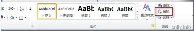
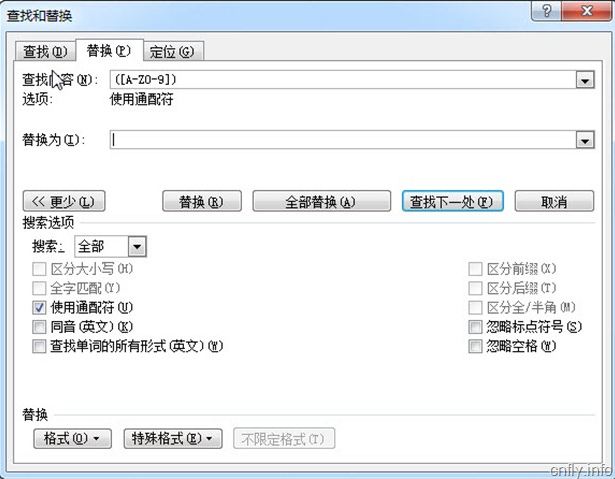
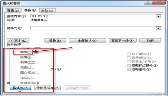
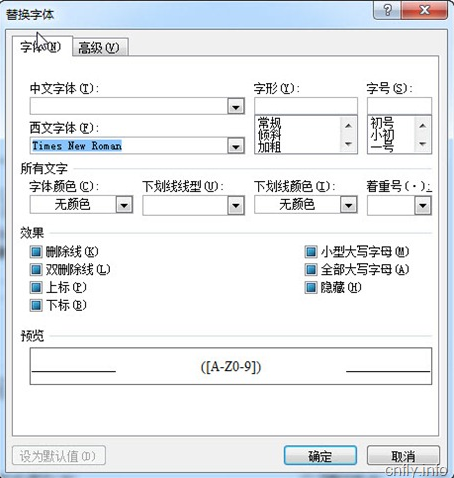
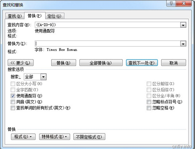
 本文介绍了一种通过使用通配符批量替换Word文档中特定字符格式的方法。具体步骤包括:使用Ctrl+H打开替换对话框,输入查找内容并启用通配符选项,选择目标字体样式,最后完成替换操作。


 1544
1544

 被折叠的 条评论
为什么被折叠?
被折叠的 条评论
为什么被折叠?
 到【灌水乐园】发言


