


本文部分代码参考github:Machine-Learning-for-Beginner-by-Python3
本文所有代码和数据集文件可在此下载:https://download.csdn.net/download/ljw_study_in_CSDN/19546447
文章目录
(一)线性回归和多项式回归
根据给定数据集,利用线性回归和多项式回归模型训练和测试一个数据预测模型,并对模型的性能和预测能力进行分析;
1. 线性回归(最小二乘法/梯度下降法)
实验代码:
import numpy as np
import pandas as pd
import matplotlib.pyplot as plt
from sklearn import preprocessing as spp  # 引入数据预处理的库
# 在训练样本集的最后一列加1
def Trans(xdata):
    ones = np.ones(len(xdata)).reshape(-1, 1)
    xta = np.append(xdata, ones, axis=1)
    return xta
# 利用传统的最小二乘法求解参数,即公式 W=(XT.X)-1*XT.Y
def ljw_leastsq(xdata, ydata):
    xdata = Trans(xdata)
    xTx = np.dot(xdata.T, xdata)
    # 判断行列式是否为零
    if np.linalg.det(xTx) == 0:
        print("the Matrix cannot do inverse!")
        return
    invert = np.linalg.inv(xTx) # 求逆阵
    ws = np.dot(np.dot(invert, xdata.T), ydata)
    return ws
# 梯度下降法
def Gradient(xdata1, ydata, learn_rate=0.1, iter_times=100000, error=1e-8):
    xdata = Trans(xdata1)
    # 系数w,b的初始化
    weights = np.zeros((xdata.shape[1], 1))  # (len(xdata[1]), 1))
    # 存储成本函数的值
    cost_function = []
    for i in range(iter_times):
        # 得到回归的值
        y_predict = np.dot(xdata, weights)
        # 最小二乘法计算误差
        cost = np.sum((y_predict - ydata) ** 2) / len(xdata)
        cost_function.append(cost)
        # 计算梯度
        dJ_dw = 2 * np.dot(xdata.T, (y_predict - ydata)) / len(xdata)
        # 更新系数w,b的值
        weights = weights - learn_rate * dJ_dw
        # 提前结束循环的机制
        if len(cost_function) > 1:
            if 0 < cost_function[-2] - cost_function[-1] < error:
                break
    return weights
def predict(xdata, ws):
    xt = Trans(xdata)
    return np.dot(xt, ws)
# 读入文本文件数据并对x进行归一化处理
def preprocess_data(filename):
    data = pd.read_table(filename, header=None).values
    x = data[:, 0].reshape(-1, 1)  # 将x由列表转化为二维数组
    y = data[:, 1].reshape(-1, 1)  # 将y由列表转化为二维数组
    x = spp.MinMaxScaler().fit_transform(x)  # 对x进行极大极小归一化
    return x, y
def draw(pic_num, fun, title):
    plt.figure(pic_num)
    w = fun(x_train, y_train)  # 用最小二乘函数或梯度下降函数,求解参数
    plt.plot(x_train, predict(x_train, w), "r", label="回归直线 $y=ax+b$")  # 拟合的直线(标为红色)
    plt.scatter(x_train, y_train, label="原数据")  # 原数据的散点图
    plt.legend()
    s = "y=" + str(round(w[0][0], 3)) + "*x+" + str(round(w[1][0], 3))  # 回归直线
    plt.text(0.05, 18, s, fontsize=20)
    plt.title(title)
    plt.show()
if __name__ == "__main__":
    x_train, y_train = preprocess_data("train.txt")
    plt.rcParams['font.sans-serif'] = 'SimSun'  # 设置中文字体
    draw(1, ljw_leastsq, "线性回归-最小二乘法拟合")
    draw(2, Gradient, "线性回归-梯度下降法拟合")
实验结果:

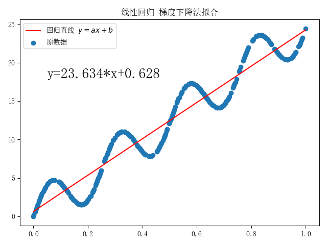
从上图可以发现,当设置梯度下降法的超参数error=1e-8时,与最小二乘法计算得到的系数w相差较小。通过不断调小参数error,梯度下降法算出的系数将更接近最小二乘法计算出的结果。
2. 多项式回归
实验代码:
import numpy as np
import pandas as pd
from scipy.optimize import leastsq
import matplotlib.pyplot as plt
# 定义多项式,w为多项式的系数
def fit_func(w, x):
    f = np.poly1d(w)  # np.ploy1d()用来构造多项式,默认 ax^3+bx^2+c^x+d
    return f(x)
# 残差函数
def err_func(w, x, y):
    ret = fit_func(w, x) - y
    return ret
# n项(最高n-1次)多项式拟合,有n个系数
def n_poly(n, x, y):
    w_init = np.random.randn(n)  # 生成n个随机数作为参数初值
    parameters = leastsq(err_func, w_init, args=(np.array(x), np.array(y)))  # 调用最小二乘法,x,y为列表型变量
    return parameters[0]
def read_data(filename):  # 读入文本文件数据
    data = pd.read_table(filename, header=None).values
    return data[:, 0], data[:, 1]
if __name__ == '__main__':
    x_train, y_train = read_data("train.txt")  # 读入数据
    x_temp = np.linspace(0, 25, 10000)  # 绘制拟合回归时需要的监测点
    row = 3
    col = 4
    plt.rcParams["font.sans-serif"] = "SimSun"  # 设置中文字体
    # 绘制子图,子图大小row*col,绘制出m次多项式的拟合回归,m设为3~14
    fig, ax = plt.subplots(row, col, figsize=(15, 10))
    m_num = row * col
    m = np.linspace(3, 3 + m_num - 1, m_num).astype(int)  # m = [3, 4, 5, 6, 7, 8, 9, 10, 11, 12, 13, 14]
    for i in range(row):
        for j in range(col):
            m_index = i * col + j
            ax[i, j].plot(x_temp, fit_func(n_poly(m[m_index] + 1, x_train, y_train), x_temp), 'r')  # 拟合的曲线(标为红色)
            ax[i, j].scatter(x_train, y_train)  # 原数据的散点图
            ax[i, j].set_title("m=" + str(m[m_index]))
            ax[i, j].legend(labels=["回归曲线", "原数据"])
    plt.show()
实验结果:
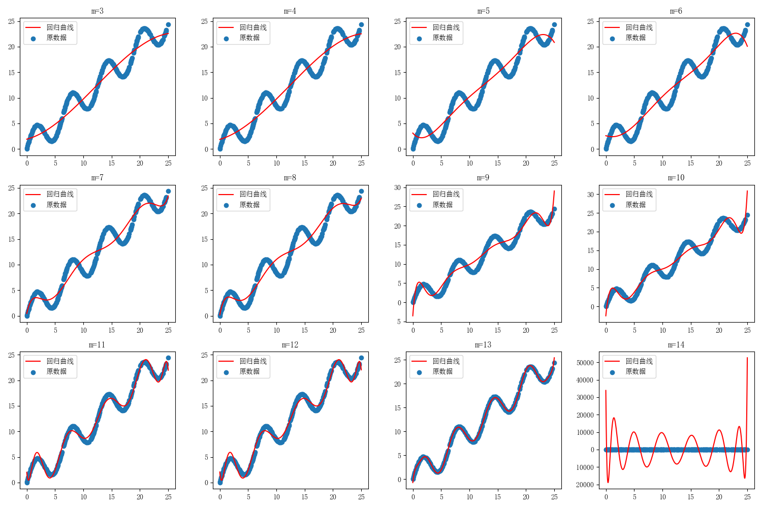
分别令最高幂次m=3,4,5,6,7,8,9,10,11,12,13,14。
从上图可以发现m=13时,多项式模型拟合效果最好。
(二)利用线性回归模型进行波斯顿房价预测
利用马萨诸塞州波士顿郊区的房屋信息数据,利用线性回归模型训练和测试一个房价预测模型,并对模型的性能和预测能力进行测试分析;
实验代码:
import numpy as np
import pandas as pd
from sklearn import preprocessing as spp # 引入数据预处理的库
import matplotlib.pyplot as plt # 绘图
from pylab import mpl
# 创建线性回归的类
class LinearRegression:
def __init__(self, learn_rate=0.2, iter_times=200000, error=1e-9):
self.learn_rate = learn_rate
self.iter_times = iter_times
self.error = error
def Trans(self, xdata):
one1 = np.ones(len(xdata))
xta = np.append(xdata, one1.reshape(-1, 1), axis=1)
return xta
# 梯度下降法
def Gradient(self, xdata, ydata):
xdata = self.Trans(xdata)
# 系数w,b的初始化
self.weights = np.zeros((len(xdata[0]), 1))
# 存储成本函数的值
cost_function = []
for i in range(self.iter_times):
# 得到回归的值
y_predict = np.dot(xdata, self.weights)
# 最小二乘法计算误差
cost = np.sum((y_predict - ydata) ** 2) / len(xdata)
cost_function.append(cost)
# 计算梯度
dJ_dw = 2 * np.dot(xdata.T, (y_predict - ydata)) / len(xdata)
# 更新系数w,b的值
self.weights = self.weights - self.learn_rate * dJ_dw
# 提前结束循环的机制
if len(cost_function) > 1:
if 0 < cost_function[-2] - cost_function[-1] < self.error:
break
return self.weights, cost_function
# 根据公式
def Formula(self, xdata, ydata):
xdata = self.Trans(xdata)
self.weights = np.dot(np.dot(np.linalg.inv(np.dot(xdata.T, xdata)), xdata.T), ydata)
y_predict = np.dot(xdata, self.weights)
cost = [np.sum((ydata - np.mean(ydata)) ** 2) / len(xdata)] # 开始是以y值得平均值作为预测值计算cost
cost += [np.sum((y_predict - ydata) ** 2) / len(xdata)] # 利用公式,一次计算便得到参数的值,不需要迭代。
return self.weights, cost # 包括2个值
# 预测
def predict(self, xdata):
return np.dot(self.Trans(xdata), self.weights)
def figure(title, *datalist):
for jj in datalist:
plt.plot(jj[0], '-', label=jj[1], linewidth=2)
plt.plot(jj[0], 'o')
plt.grid()
plt.title(title)
plt.legend()
plt.show()
# 计算R2的函数
def getR(ydata_tr, ydata_pre):
sum_error = np.sum(((ydata_tr - np.mean(ydata_tr)) ** 2))
inexplicable = np.sum(((ydata_tr - ydata_pre) ** 2))
return 1 - inexplicable / sum_error
# 读取数据并进行数据预处理
def preprocess_data(percent=0.1):
data = pd.read_csv(r'Boston.csv')
xdata = data.drop('MEDV', axis=1).values
xdata = spp.MinMaxScaler().fit_transform(xdata) # 归一的x值,y值分为训练数据集和预测数据集
ydata = data['MEDV']
sign_list = list(range(len(xdata)))
# 用于测试的序号
select_sign = sorted(np.random.choice(sign_list, int(len(xdata) * percent), replace=False))
# 用于训练的序号
no_select_sign = [isign for isign in sign_list if isign not in select_sign]
# 测试数据
x_predict_data = xdata[select_sign]
y_predict_data = ydata[select_sign].values.reshape(len(select_sign), 1) # 转化数据结构
# 训练数据
x_train_data = xdata[no_select_sign]
y_train_data = ydata[no_select_sign].values.reshape(len(no_select_sign), 1) # 转化数据结构
return x_train_data, y_train_data, x_predict_data, y_predict_data # 训练集、测试集
if __name__ == "__main__":
regressor = LinearRegression()
lrdata = preprocess_data() # 可用于算法的数据
train_error = regressor.Gradient(lrdata[0], lrdata[1]) # 开始训练
predict_result = regressor.predict(lrdata[2]) # 用于预测数据的预测值
train_pre_result = regressor.predict(lrdata[0]) # 用于训练数据的预测值
mpl.rcParams['font.sans-serif'] = ['SimHei'] # 设置中文字体
mpl.rcParams['axes.unicode_minus'] = False
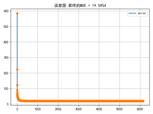
figure('误差图 最终的MSE = %.4f' % (train_error[1][-1]), [train_error[1], 'error']) # 绘制误差图
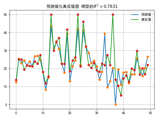
figure('预测值与真实值图 模型的' + r'$R^2=%.4f$' % (getR(lrdata[1], train_pre_result)), [predict_result, '预测值'],
[lrdata[3], '真实值']) # 绘制预测值与真实值图
plt.show()
print('线性回归的系数为:\n w = %s, \nb= %s' % (train_error[0][:-1], train_error[0][-1]))
实验结果:
(三)利用logistic回归模型进行心脏病预测
心脏病是人类健康的头号杀手。全世界1/3的人口死亡是因心脏病引起的,而我国,每年有几十万人死于心脏病。 所以,如果可以通过提取人体相关的体侧指标,通过数据挖掘的方式来分析不同特征对于心脏病的影响,对于预测和预防心脏病将起到至关重要的作用。本文将会通过真实的数据,通过Python搭建心脏病预测案例。
实验代码:
import numpy as np
import pandas as pd
from prettytable import PrettyTable # 用于计算混淆矩阵
import matplotlib.pyplot as plt
from pylab import mpl
def confusion(realy, outy):
mix = PrettyTable()
type = sorted(list(set(realy.T[0])), reverse=True)
mix.field_names = [' '] + ['预测:%d类' % si for si in type]
# 字典形式存储混淆矩阵数据
cmdict = {}
for jkj in type:
cmdict[jkj] = []
for hh in type:
hu = len(['0' for jj in range(len(realy)) if realy[jj][0] == jkj and outy[jj][0] == hh])
cmdict[jkj].append(hu)
# 输出表格
for fu in type:
mix.add_row(['真实:%d类' % fu] + cmdict[fu])
return mix
# 返回混淆矩阵用到的数据TP,TN,FP,FN
def getmatrix(realy, outy, possclass=1): # 默认类1 为正类
TP = len(['0' for jj in range(len(realy)) if realy[jj][0] == possclass and outy[jj][0] == possclass]) # 实际正预测正
TN = len(
['0' for jj in range(len(realy)) if realy[jj][0] == 1 - possclass and outy[jj][0] == 1 - possclass]) # 实际负预测负
FP = len(['0' for jj in range(len(realy)) if realy[jj][0] == 1 - possclass and outy[jj][0] == possclass]) # 实际负预测正
FN = len(['0' for jj in range(len(realy)) if realy[jj][0] == possclass and outy[jj][0] == 1 - possclass]) # 实际正预测负
# 假正率
FPR = FP / (FP + TN)
# 真正率
TPR = TP / (TP + FN)
return FPR, TPR
class LRReg:
def __init__(self, learn_rate=0.5, iter_times=40000, error=1e-9, cpn='L2'):
self.learn_rate = learn_rate
self.iter_times = iter_times
self.error = error
self.cpn = cpn
# w和b合为一个参数,也就是x最后加上一列全为1的数据。
def trans(self, xdata):
one1 = np.ones(len(xdata))
xta = np.append(xdata, one1.reshape(-1, 1), axis=1)
return xta
# 梯度下降法
def Gradient(self, xdata, ydata, func=trans):
xdata = func(self, xdata)
# 系数w,b的初始化
self.weights = np.zeros((len(xdata[0]), 1))
# 存储成本函数的值
cost_function = []
for i in range(self.iter_times):
# 得到回归的值
y_predict = np.dot(xdata, self.weights)
# Sigmoid函数的值
s_y_pre = 1 / (1 + np.exp(-y_predict))
# 计算最大似然的值
like = np.sum(np.dot(ydata.T, np.log(s_y_pre)) + np.dot((1 - ydata).T, np.log(1 - s_y_pre)))
# 正则化
if self.cpn == 'L2':
# 成本函数中添加系数的L2范数
l2norm = np.sum(0.5 * np.dot(self.weights.T, self.weights) / len(xdata))
cost = -like / len(xdata) + l2norm
grad_W = np.dot(xdata.T, (s_y_pre - ydata)) / len(xdata) + 0.9 * self.weights / len(xdata)
else:
cost = -like / (len(xdata))
grad_W = np.dot(xdata.T, (s_y_pre - ydata)) / len(xdata)
cost_function.append(cost)
print(cost, like)
# 训练提前结束
if len(cost_function) > 2:
if 0 <= cost_function[-1] - cost_function[-2] <= self.error:
break
# 更新
self.weights = self.weights - self.learn_rate * grad_W
return self.weights, cost_function
# 预测
def predict(self, xdata, func=trans, yuzhi=0.5):
pnum = np.dot(func(self, xdata), self.weights)
s_pnum = 1 / (1 + np.exp(-pnum))
latnum = [[1] if jj[0] >= yuzhi else [0] for jj in s_pnum]
return latnum
# 开始进行数据处理【没有缺失值】
def preprocess_data():
data = pd.read_csv(r'./Heart.csv')
normal = [1, 4, 5, 8, 10, 12, 11] # 标准化处理
one_hot = [3, 7, 13] # one_hot编码
binary = [14] # 原始类别为1的依然为1类,原始为2的变为0类
keylist = data.keys()
newexdata = pd.DataFrame()
for ikey in range(len(keylist)):
if ikey + 1 in normal:
newexdata[keylist[ikey]] = (data[keylist[ikey]] - data[keylist[ikey]].mean()) / data[keylist[ikey]].std()
elif ikey + 1 in binary:
newexdata[keylist[ikey]] = [1 if inum == 1 else 0 for inum in data[keylist[ikey]]]
elif ikey + 1 in one_hot:
newdata = pd.get_dummies(data[keylist[ikey]], prefix=keylist[ikey])
newexdata = pd.concat([newexdata, newdata], axis=1)
x_pre_data = newexdata.values[:, :-1]
y_data = newexdata.values[:, -1].reshape(-1, 1)
return x_pre_data, y_data
if __name__ == "__main__":
lr_re = LRReg()
H_Data = preprocess_data() # 最终的可用于算法的数据
lf = lr_re.Gradient(H_Data[0], H_Data[1])
print('系数为:\n', lr_re.weights)
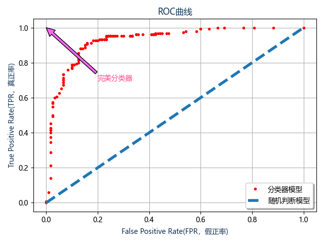
# 绘制ROC曲线
yuzi = np.linspace(0, 1, 101) # 从0到1定义不同的阈值
roc = [] # ROC 曲线数据
for yy in yuzi: # 开始遍历不同的阈值
fdatd = lr_re.predict(H_Data[0], yuzhi=yy)
if yy == 0.5:
print('阈值为%s时的混淆矩阵:\n' % yy, confusion(H_Data[1], fdatd))
roc.append(getmatrix(H_Data[1], fdatd))
fu = np.array(sorted(roc, key=lambda x: x[0])) # 首线是FPR按着从小到大排列
# 开始绘制ROC曲线图
mpl.rcParams['font.sans-serif'] = ['Microsoft Yahei'] # 作图显示中文
fig, ax1 = plt.subplots()
ax1.plot(list(fu[:, 0]), list(fu[:, 1]), '.', linewidth=4, color='r')
ax1.plot([0, 1], '--', linewidth=4)
ax1.grid('on')
ax1.legend(['分类器模型', '随机判断模型'], loc='lower right', shadow=True, fontsize='medium')
ax1.annotate('完美分类器', xy=(0, 1), xytext=(0.2, 0.7), color='#FF4589', arrowprops=dict(facecolor='#FF67FF'))
ax1.set_title('ROC曲线', color='#123456')
ax1.set_xlabel('False Positive Rate(FPR,假正率)', color='#123456')
ax1.set_ylabel('True Positive Rate(TPR,真正率)', color='#123456')
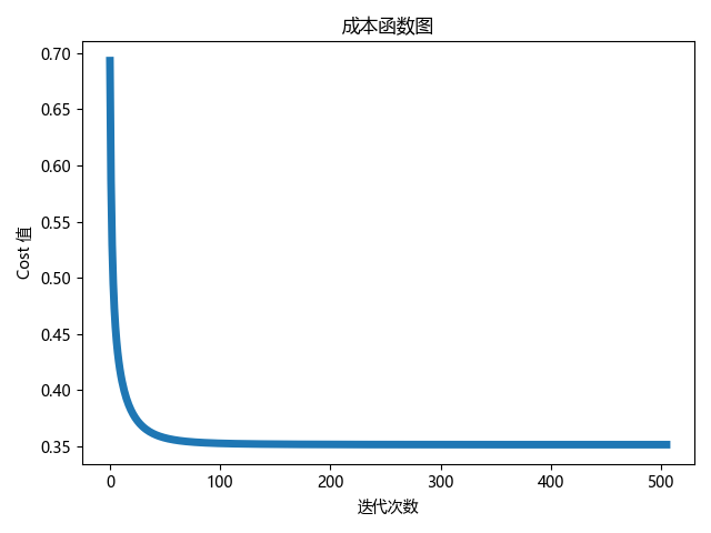
# 绘制成本函数图
fig, ax2 = plt.subplots()
ax2.plot(list(range(len(lf[1]))), lf[1], '-', linewidth=5)
ax2.set_title('成本函数图')
ax2.set_ylabel('Cost 值')
ax2.set_xlabel('迭代次数')
plt.show()
实验结果:
系数为:
 [[ 0.22442019]
 [ 0.66719841]
 [ 0.07366912]
 [ 0.60077063]
 [-1.13520668]
 [-0.32244956]
 [-0.16243874]
 [ 0.42651962]
 [ 0.01357678]
 [-0.23366492]
 [ 0.49654308]
 [-0.55760351]
 [-0.22314746]
 [-1.02066971]
 [ 0.94635202]
 [ 0.20900704]
 [-0.94892758]
 [ 0.20643148]]
阈值为0.5时的混淆矩阵:
 +----------+----------+----------+
|          | 预测:1类 | 预测:0类 |
+----------+----------+----------+
| 真实:1类 |   140    |    10    |
| 真实:0类 |    25    |    95    |
+----------+----------+----------+
(四)利用softmax回归进行莺尾花分类预测
softmax回归是logistic回归的推广,通过独热向量表示类别,使用交叉熵损失函数来学习最优的参数矩阵W,对样本进行多分类(对Iris数据集进行三分类)。
实验代码:
import numpy as np
import pandas as pd
import matplotlib.pyplot as plt
from pylab import mpl
from prettytable import PrettyTable  # 用于计算混淆矩阵
class LRReg:
    def __init__(self, learn_rate=0.9, iter_times=40000, error=1e-17):
        self.learn_rate = learn_rate
        self.iter_times = iter_times
        self.error = error
    # w和b合为一个参数,也就是x最后加上一列全为1的数据
    def trans(self, xdata):
        one1 = np.ones(len(xdata))
        xta = np.append(xdata, one1.reshape(-1, 1), axis=1)
        return xta
    # 梯度下降法
    def Gradient(self, xdata, ydata, func=trans):
        xdata = func(self, xdata)
        # 系数w,b的初始化
        self.weights = np.zeros((len(xdata[0]), len(ydata[0])))
        # 存储成本函数的值
        cost_function = []
        for i in range(self.iter_times):
            # 计算np.exp(X.W)的值
            exp_xw = np.exp(np.dot(xdata, self.weights))
            # 计算y_predict每一行的和值
            sumrow = np.sum(exp_xw, axis=1).reshape(-1, 1)
            # 计算除去和值得值
            devi_sum = exp_xw / sumrow
            # 计算减法
            sub_y = ydata - devi_sum
            # 得到梯度
            grad_W = -1 / len(xdata) * np.dot(xdata.T, sub_y)
            # 正则化,成本函数中添加系数的L2范数
            l2norm = np.sum(0.5 * np.dot(self.weights.T, self.weights) / len(xdata))
            last_grad_W = grad_W + 0.002 * self.weights / len(xdata)
            # 计算最大似然的对数的值
            likehood = np.sum(ydata * devi_sum)
            cost = - likehood / len(xdata) + l2norm
            cost_function.append(cost)
            # 训练提前结束
            if len(cost_function) > 2:
                if 0 <= cost_function[-2] - cost_function[-1] <= self.error:
                    break
            # 更新
            self.weights = self.weights - self.learn_rate * last_grad_W
        return self.weights, cost_function
    # 预测
    def predict(self, xdata, func=trans):
        pnum = np.dot(func(self, xdata), self.weights)
        # 选择每一行中最大的数的index
        maxnumber = np.max(pnum, axis=1)
        # 预测的类别
        y_pre_type = []
        for jj in range(len(maxnumber)):
            fu = list(pnum[jj]).index(maxnumber[jj]) + 1
            y_pre_type.append([fu])
        return np.array(y_pre_type)
# 将独热编码的类别变为标识为1,2,3的类别
def transign(eydata):
    ysign = []
    for hh in eydata:
        ysign.append([list(hh).index(1) + 1])
    return np.array(ysign)
def confusion(realy, outy, method='AnFany'):
    mix = PrettyTable()
    type = sorted(list(set(realy.T[0])), reverse=True)
    mix.field_names = [method] + ['预测:%d类' % si for si in type]
    # 字典形式存储混淆矩阵数据
    cmdict = {}
    for jkj in type:
        cmdict[jkj] = []
        for hh in type:
            hu = len(['0' for jj in range(len(realy)) if realy[jj][0] == jkj and outy[jj][0] == hh])
            cmdict[jkj].append(hu)
    # 输出表格
    for fu in type:
        mix.add_row(['真实:%d类' % fu] + cmdict[fu])
    return mix
# setosa  [1,0,0]
# versicolor [0,1,0]
# virginica  [0,0,1]
def preprocess_data():
    data = pd.read_csv(r'iris.csv')
    xdata = data.iloc[:, 1:5].values  # x值
    handle_x_data = (xdata - np.mean(xdata, axis=0)) / np.std(xdata, axis=0) # x数据标准化
    ydata = pd.get_dummies(data['Species']).values  # y数据独热化
    xydata = np.hstack((handle_x_data, ydata))  # 首先将x数据和y数据合在一起
    np.random.shuffle(xydata)  # 因为数据中类别比较集中,不易于训练,因此打乱数据
    return xydata[:, :4], xydata[:, 4:]
if __name__ == '__main__':
    lr_re = LRReg()
    data = preprocess_data()
    lf = lr_re.Gradient(data[0], data[1])
    y_calss_pre = lr_re.predict(data[0])
    print('系数:\n', lr_re.weights)
    print('混淆矩阵:\n', confusion(transign(data[1]), y_calss_pre))
    # 绘制成本函数图
    mpl.rcParams['font.sans-serif'] = ['FangSong']  # 设置中文字体新宋体(作图显示中文)
    mpl.rcParams['axes.unicode_minus'] = False
    plt.plot(list(range(len(lf[1]))), lf[1], '-', linewidth=5)
    plt.title('成本函数图')
    plt.ylabel('Cost 值')
    plt.xlabel('迭代次数')
    plt.show()
实验结果:
系数:
 [[-3.18259494  2.53486939  0.64772555]
 [ 3.21960963 -0.39859444 -2.82101519]
 [-7.12327144 -3.49716456 10.620436  ]
 [-6.67192748 -2.51948539  9.19141287]
 [ 0.16517529  8.35513963 -8.52031491]]
混淆矩阵:
+----------+----------+----------+----------+
|  AnFany  | 预测:3类 | 预测:2类 | 预测:1类  |
+----------+----------+----------+----------+
| 真实:3类 |    49    |    1     |    0     |
| 真实:2类 |    1     |    49    |    0     |
| 真实:1类 |    0     |    0     |    50    |
+----------+----------+----------+----------+


 575
575


 被折叠的 条评论
为什么被折叠?
被折叠的 条评论
为什么被折叠?
 到【灌水乐园】发言


