


目录
- 一、实验原理(Transformer)
- 二、Japanese-Chinese Machine Translation Model with Transformer & PyTorch
- 2.1 Import required packages
- 2.2 Get the parallel dataset
- 2.3 Prepare the tokenizers
- 2.4 Build the TorchText Vocab objects and convert the sentences into Torch tensors
- 2.5 Create the DataLoader object to be iterated during training
- 2.6 Sequence-to-sequence Transformer
- 2.7 Start training
- 2.8 Try translating a Japanese sentence using the trained model
- 2.9 Save the Vocab objects and trained model
- 三、实验总结
- 四、参考文献
一、实验原理(Transformer)
1.1 Transformer是什么
Transformer是一种用于自然语言处理(NLP)和其他序列到序列(sequence-to-sequence)任务的深度学习模型架构,它在2017年由Vaswani等人首次提出。Transformer架构引入了自注意力机制(self-attention mechanism),这是一个关键的创新,使其在处理序列数据时表现出色。
以下是Transformer的一些重要组成部分和特点:
- 自注意力机制(Self-Attention):这是Transformer的核心概念之一,它使模型能够同时考虑输入序列中的所有位置,而不是像循环神经网络(RNN)或卷积神经网络(CNN)一样逐步处理。自注意力机制允许模型根据输入序列中的不同部分来赋予不同的注意权重,从而更好地捕捉语义关系。
- 多头注意力(Multi-Head Attention):Transformer中的自注意力机制被扩展为多个注意力头,每个头可以学习不同的注意权重,以更好地捕捉不同类型的关系。多头注意力允许模型并行处理不同的信息子空间。
- 堆叠层(Stacked Layers):Transformer通常由多个相同的编码器和解码器层堆叠而成。这些堆叠的层有助于模型学习复杂的特征表示和语义。
- 位置编码(Positional Encoding):由于Transformer没有内置的序列位置信息,它需要额外的位置编码来表达输入序列中单词的位置顺序。
- 残差连接和层归一化(Residual Connections and Layer Normalization):这些技术有助于减轻训练过程中的梯度消失和爆炸问题,使模型更容易训练。
- 编码器和解码器:Transformer通常包括一个编码器用于处理输入序列和一个解码器用于生成输出序列,这使其适用于序列到序列的任务,如机器翻译。
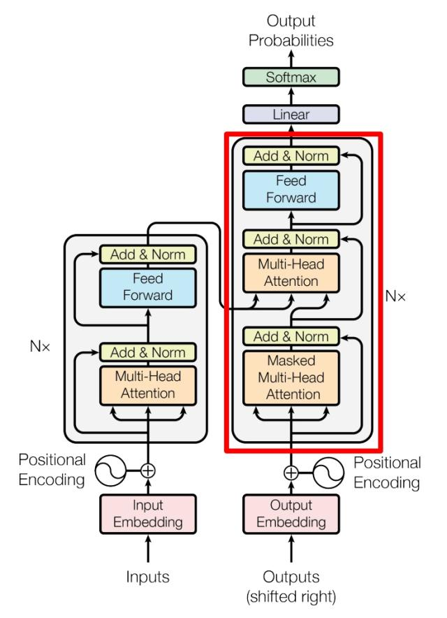
1.2 Transformer整体结构
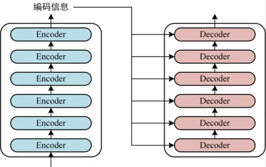
可以看到 Transformer由Encoder和Decoder两个部分组成,Encoder和Decoder都包含 6 个 block。Transformer的工作流程大体如下:
第一步:获取输入句子的每一个单词的表示向量 X X X, X X X由单词的Embedding(Embedding就是从原始数据提取出来的Feature) 和单词位置的 Embedding 相加得到。
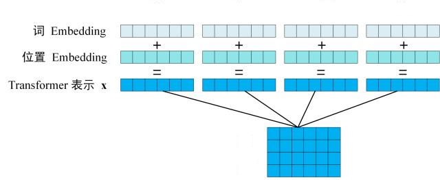
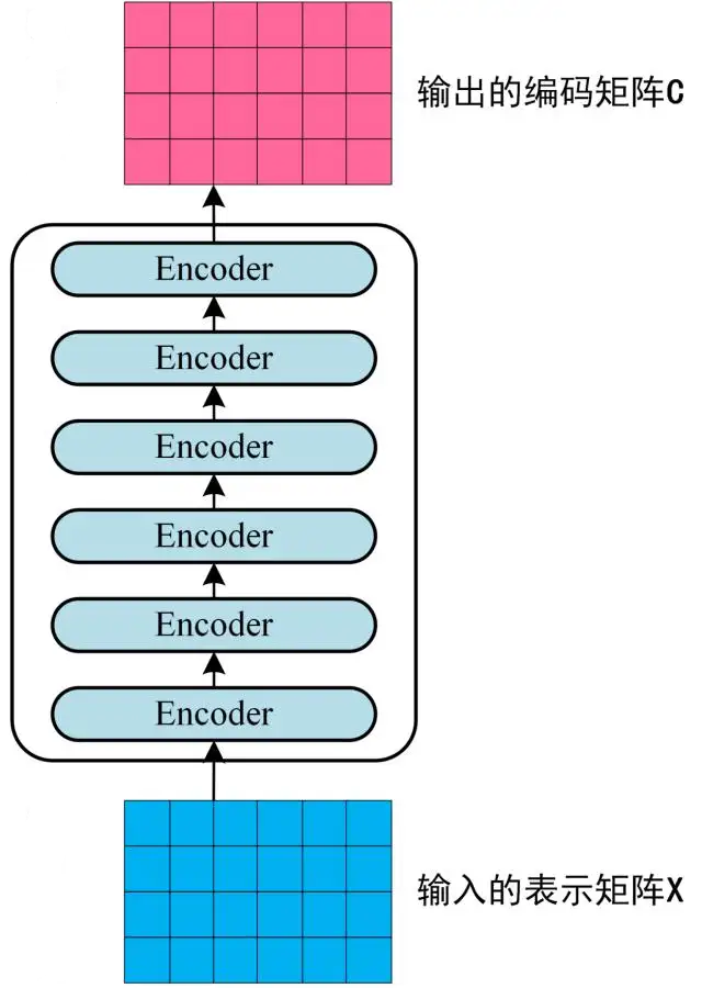
第二步:将得到的单词表示向量矩阵 (如上图所示,每一行是一个单词的表示 x x x) 传Encoder中,经过 6 个Encoder block后可以得到句子所有单词的编码信息矩阵 C C C,如下图。单词向量矩阵用 表示, n n n是句子中单词个数, d d d是表示向量的维度 (论文中 d d d=512)。每一个Encoder block输出的矩阵维度与输入完全一致。

第三步:将 Encoder输出的编码信息矩阵 C C C传递到Decoder中,Decoder依次会根据当前翻译过的单词 1~ i 翻译下一个单词 i + 1 i+1 i+1,如下图所示。在使用的过程中,翻译到单词 i + 1 i+1 i+1的时候需要通过 Mask (掩盖) 操作遮盖住 i + 1 i+1 i+1之后的单词。
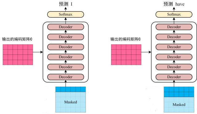
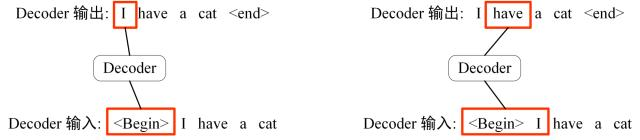
上图Decoder接收了Encoder编码矩阵 C C C,然后首先输入一个翻译开始符 “”,预测第一个单词 “I”;然后输入翻译开始符 “” 和单词 “I”,预测单词 “have”,以此类推。这是Transformer使用时候的大致流程,接下来是里面各个部分的细节。
1.3 Transformer的输入
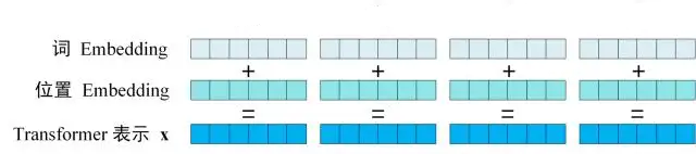
Transformer中单词的输入表示 x x x由单词Embedding 和位置Embedding (Positional Encoding)相加得到。
1.3.1 单词Embedding
单词的Embedding有很多种方式可以获取,例如可以采用Word2Vec、Glove等算法预训练得到,也可以在Transformer中训练得到。
1.3.2 位置Embedding
Transformer中除了单词的Embedding,还需要使用位置Embedding表示单词出现在句子中的位置。**因为Transformer不采用RNN的结构,而是使用全局信息,不能利用单词的顺序信息,而这部分信息对于NL 来说非常重要。**所以Transformer中使用位置Embedding保存单词在序列中的相对或绝对位置。
位置Embedding用 PE表示,PE的维度与单词 Embedding是一样的。PE 可以通过训练得到,也可以使用某种公式计算得到。在Transformer中采用了后者,计算公式如下:
P
E
(
p
o
i
,
2
i
)
=
sin
(
p
o
i
/
1000
0
2
i
/
d
)
P
E
(
p
o
i
,
2
i
+
1
)
=
cos
(
p
o
i
/
1000
0
2
i
/
d
)
PE_{(poi,2i)}=\sin(poi/10000^{2i/d})\\ PE_{(poi,2i+1)}=\cos(poi/10000^{2i/d})
PE(poi,2i)=sin(poi/100002i/d)PE(poi,2i+1)=cos(poi/100002i/d)
- 使PE能够适应比训练集里面所有句子更长的句子,假设训练集里面最长的句子是有20个单词,突然来了一个长度为21的句子,则使用公式计算的方法可以计算出第21位的Embedding。
- 可以让模型容易地计算出相对位置,对于固定长度的间距 k k k, P E ( p o s + k ) PE(pos+k) PE(pos+k)可以用 P E ( p o s ) PE(pos) PE(pos) 计算得到。因为 sin ( A + B ) = sin ( A ) C o s ( B ) + cos ( A ) sin ( B ) , cos ( A + B ) = cos ( A ) cos ( B ) − sin ( A ) sin ( B ) \sin(A+B)=\sin(A)Cos(B)+\cos(A)\sin(B),\cos(A+B)=\cos(A)\cos(B)-\sin(A)\sin(B) sin(A+B)=sin(A)Cos(B)+cos(A)sin(B),cos(A+B)=cos(A)cos(B)−sin(A)sin(B)。
1.4 Self-Attention(自注意力机制)
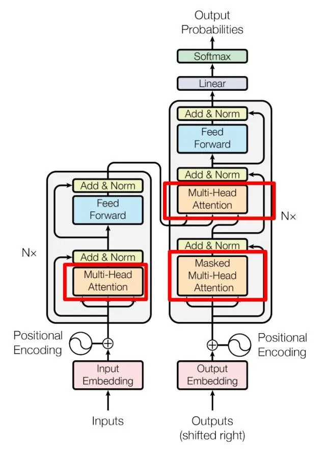
上图是论文中Transformer的内部结构图,左侧为Encoder block,右侧为Decoder block。红色圈中的部分为Multi-Head Attention,是由多个Self-Attention组成的,可以看到Encoder block 包含一个Multi-Head Attention,而Decoder block包含两个Multi-Head Attention(其中有一个用到Masked)。Multi-Head Attention上方还包括一个Add & Norm层,Add表示残差连接 (Residual Connection) 用于防止网络退化,Norm表示Layer Normalization,用于对每一层的激活值进行归一化。
1.4.1 Self-Attention 结构
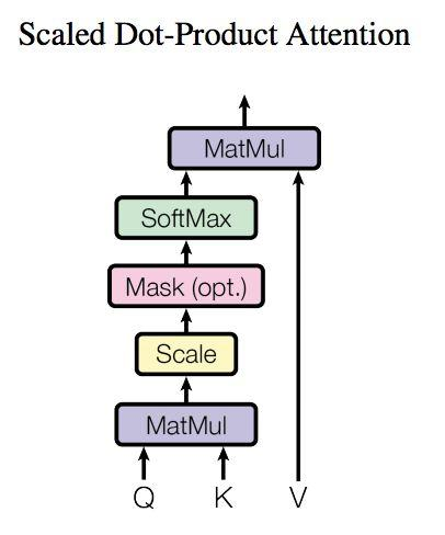
上图是Self-Attention的结构,在计算的时候需要用到矩阵 Q Q Q(查询), K K K(键值), V V V(值)。在实际中,Self-Attention接收的是输入(单词的表示向量x组成的矩阵 X X X) 或者上一个Encoder block的输出。而 Q , K , V Q,K,V Q,K,V正是通过Self-Attention的输入进行线性变换得到的。
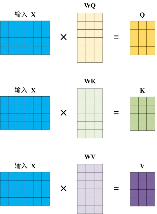
1.4.2 Q Q Q, K K K, V V V的计算
Self-Attention的输入用矩阵X进行表示,则可以使用线性变阵矩阵 W Q , W K , W V WQ,WK,WV WQ,WK,WV计算得到 Q , K , V Q,K,V Q,K,V。计算如下图所示,注意 X , Q , K , V X,Q,K,V X,Q,K,V的每一行都表示一个单词。
1.4.3 Self-Attention的输出
得到矩阵
Q
,
K
,
V
Q, K, V
Q,K,V之后就可以计算出Self-Attention的输出了,计算的公式如下:
A
t
t
e
n
t
i
o
n
(
Q
,
K
,
V
)
=
s
o
f
t
m
a
x
(
Q
K
⊤
d
k
)
V
Attention(Q,K,V)=softmax\left(\frac{QK^\top}{\sqrt{d_k}}\right)V
Attention(Q,K,V)=softmax(dkQK⊤)V
公式中计算矩阵
Q
Q
Q和
K
K
K每一行向量的内积,为了防止内积过大,因此除以
d
k
d_k
dk的平方根。
Q
Q
Q乘以
K
K
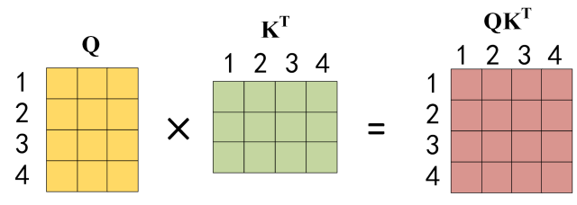
K的转置后,得到的矩阵行列数都为
n
n
n,
n
n
n为句子单词数,这个矩阵可以表示单词之间的attention强度。下图为
Q
Q
Q乘以
K
⊤
K^\top
K⊤ ,1234表示的是句子中的单词。
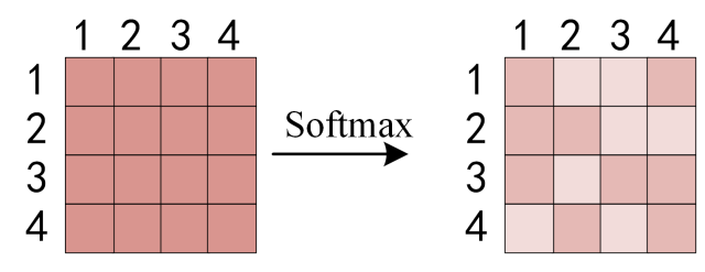
得到 Q K ⊤ QK^\top QK⊤ 之后,使用Softmax计算每一个单词对于其他单词的attention系数,公式中的Softmax是对矩阵的每一行进行Softmax,即每一行的和都变为1。
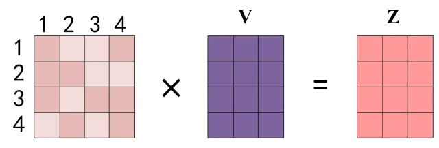
到Softmax矩阵之后可以和 V V V相乘,得到最终的输出 Z Z Z。
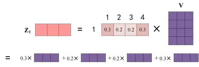
上图中Softmax矩阵的第1行表示单词1与其他所有单词的attention系数,最终单词1的输出 Z 1 Z_1 Z1等于所有单词 i i i的值得到8个输出矩阵之后,Multi-Head Attention将它们拼接在一起**(Concat),然后传入一个Linear**层,得到Multi-Head Attention最终的输出 Z Z Z。 根据attention系数的比例加在一起得到,如下图所示:
1.4.4 Multi-Head Attention
Multi-Head Attention是由多个Self-Attention组合形成的,下图是论文中Multi-Head Attention的结构图。
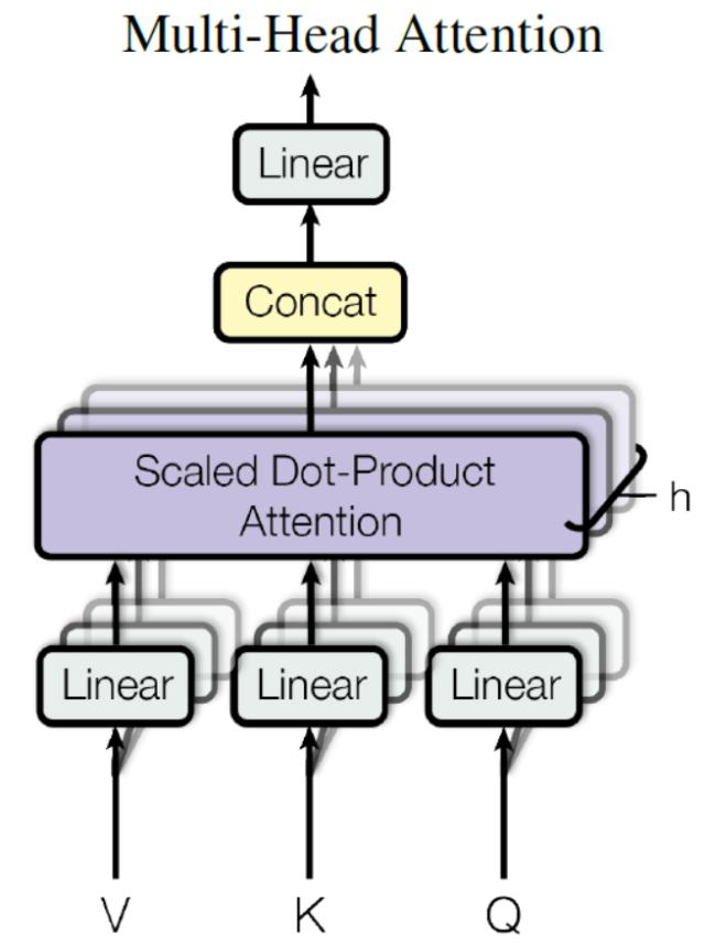
从上图可以看到Multi-Head Attention包含多个Self-Attention层,首先将输入 X X X分别传递到 h h h个不同的Self-Attention中,计算得到 h h h个输出矩阵 Z Z Z。下图是 h = 8 h=8 h=8时候的情况,此时会得到 8 8 8个输出矩阵 Z Z Z。
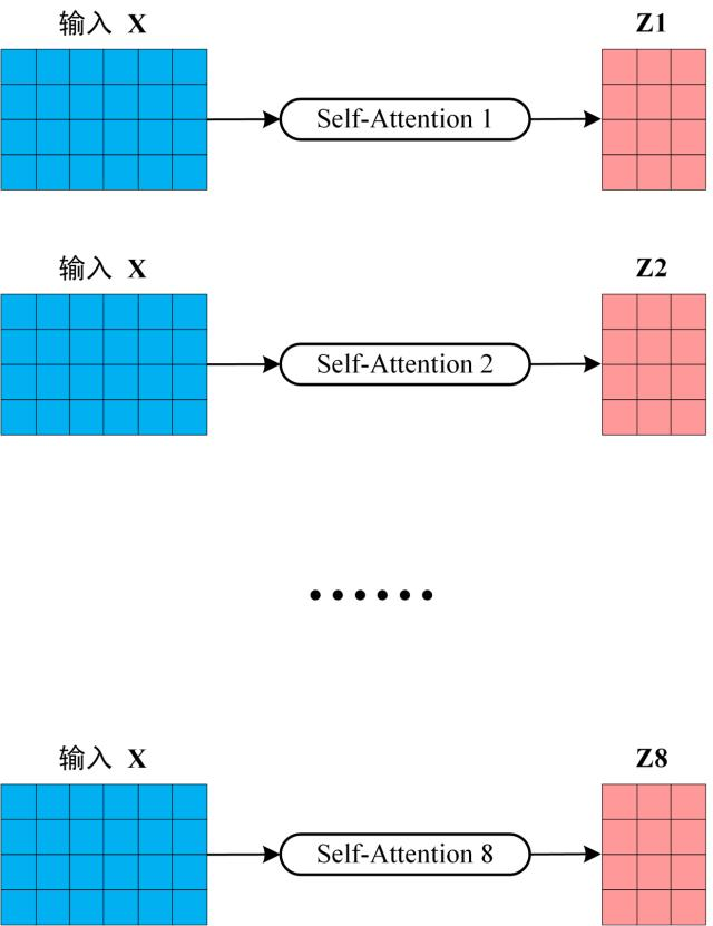
得到8个输出矩阵 Z 1 Z_1 Z1 到 Z 8 Z_8 Z8之后,Multi-Head Attention将它们拼接在一起 (Concat),然后传入一个Linear层,得到Multi-Head Attention最终的输出 Z Z Z。
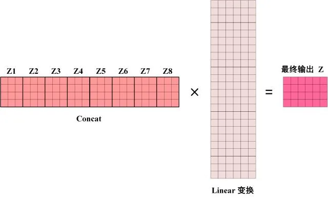
可以看到Multi-Head Attention输出的矩阵 Z Z Z与其输入的矩阵 X X X的维度是一样的。
1.5 Encoder 结构
上图红色部分是Transformer的Encoder block结构,可以看到是由Multi-Head Attention, Add & Norm, Feed Forward, Add & Norm组成的。刚刚已经了解了Multi-Head Attention的计算过程,现在了解一下Add & Norm和Feed Forward部分。
1.5.1 Add & Norm
Add & Norm 层由Add和Norm两部分组成,其计算公式如下:
L
a
y
e
r
N
o
r
m
=
(
X
+
M
u
l
t
i
H
e
a
d
A
t
t
e
n
t
i
o
n
(
X
)
)
L
a
y
e
r
N
o
r
m
(
X
+
F
e
e
d
F
o
r
w
a
r
d
(
X
)
)
LayerNorm=(X+MultiHeadAttention(X))\\ LayerNorm(X+FeedForward(X))
LayerNorm=(X+MultiHeadAttention(X))LayerNorm(X+FeedForward(X))
其中
X
X
X表示Multi-Head Attention或者Feed Forward的输入,MultiHeadAttention(
X
X
X)和FeedForward(X)表示输出(输出与输入
X
X
X维度是一样的,所以可以相加)。
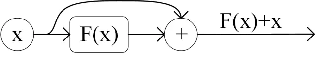
Add指X+MultiHeadAttention(X),是一种残差连接,通常用于解决多层网络训练的问题,可以让网络只关注当前差异的部分,在ResNet中经常用到:
Norm指Layer Normalization,通常用于RNN结构,Layer Normalization会将每一层神经元的输入都转成均值方差都一样的,这样可以加快收敛。
1.5.2 Feed Forward
Feed Forward层比较简单,是一个两层的全连接层,第一层的激活函数为Relu,第二层不使用激活函数,对应的公式如下:
max
(
0
,
X
W
1
+
b
1
)
W
2
+
b
2
\max{(0,XW_1+b_1)}W_2+b_2
max(0,XW1+b1)W2+b2
X
X
X是输入,Feed Forward最终得到的输出矩阵的维度与
X
X
X一致。
1.5.3 组成 Encoder
通过上面描述的Multi-Head Attention, Fed Forward, Add & Norm就可以造出一个Encoder block,Encoder block接收输入矩阵 X ( n × d ) X_{(n×d)} X(n×d) ,并输出一个矩阵 = O ( n × d ) O_{(n×d)} O(n×d) 。通过多个Encoder block叠加就可以组成 Encoder。
第一 个Encoder block的输入为句子单词的表示向量矩阵,后续Encoder block的输入是前一个Encoder block的输出,最后一个Encoder block输出的矩阵就是编码信息矩阵 C C C,这一矩阵后续会用到Decoder中。
1.6 Decoder 结构
上图红色部分为Transformer的Decoder block结构,与Encoder block相似,但是存在一些区别:
- 包含两个Multi-Head Attention层。
- 第一个Multi-Head Attention层采用了Masked操作。
- 第二个Multi-Head Attention层的 K , V K, V K,V矩阵使用Encoder的**编码信息矩阵 C C C**进行计算,而Q使用上一个Decoder block的输出计算。
- 最后有一个 Softmax 层计算下一个翻译单词的概率。
1.6.1 第一个Multi-Head Attention
Decoder block 的第一个 Multi-Head Attention 采用了 Masked 操作,因为在翻译的过程中是顺序翻译的,即翻译完第 i 个单词,才可以翻译第 i+1 个单词。通过 Masked 操作可以防止第 i 个单词知道 i+1 个单词之后的信息。下面以 “我有一只猫” 翻译成 “I have a cat” 为例,了解一下 Masked 操作。
下面的描述中使用了类似 Teacher Forcing 的概念,不熟悉 Teacher Forcing 的童鞋可以参考以下上一篇文章Seq2Seq 模型详解。在 Decoder 的时候,是需要根据之前的翻译,求解当前最有可能的翻译,如下图所示。首先根据输入 “Begin” 预测出第一个单词为 “I”,然后根据输入 “Begin I” 预测下一个单词 “have”。
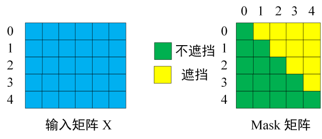
Decoder可以在训练的过程中使用Teacher Forcing并且并行化训练,即将正确的单词序列 ( I have a cat) 和对应输出 (I have a cat ) 传递到Decoder。那么在预测第 i i i个输出时,就要将第 i + 1 i+1 i+1之后的单词掩盖住,注意Mask操作是在Self-Attention的Softmax之前使用的,下面用 0 1 2 3 4 5 分别表示 " I have a cat "。
第一步:是Decoder的输入矩阵和Mask矩阵,输入矩阵包含 " I have a cat" (0, 1, 2, 3, 4) 五个单词的表示向量,Mask是一个 5×5 的矩阵。在Mask可以发现单词0只能使用单词0 信息,而单词1可以使用单词0, 1的信息,即只能使用之前的信息。
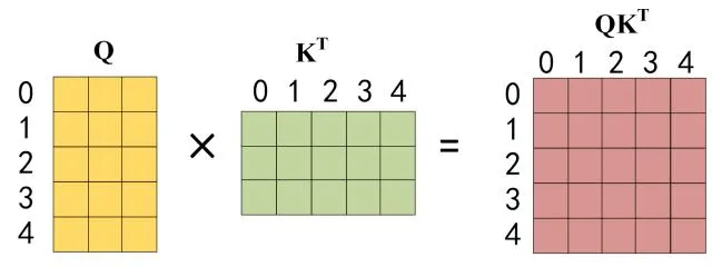
第二步: 接下来的操作和之前的Self-Attention一样,通过输入矩阵 X X X计算得到 Q , K , V Q,K,V Q,K,V矩阵。然后计算 Q Q Q和 K T K^T KT的乘积 Q K T QK^T QKT 。
第三步: 在得到 之后需要进行Softmax,计算attention score,我们在Softmax之前需要使用Mask矩阵遮挡住每一个单词之后的信息,遮挡操作如下:
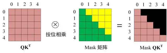
得到 Mask Q K T QK^T QKT之后在 Mask Q K T QK^T QKT上进行Softmax,每一行的和都为1。但是单词0在单词1, 2, 3, 4上的attention score都为0。
**第四步:**使用 Mask Q K T QK^T QKT与矩阵V相乘,得到输出 Z Z Z,则单词1的输出向量 Z 1 Z_1 Z1 是只包含单词1信息的。
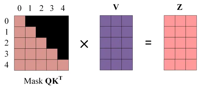
第五步: 通过上述步骤就可以得到一个Mask Self-Attention的输出矩阵 Z i Z_i Zi ,然后和Encoder类似,通过Multi-Head Attention拼接多个输出 Z i Z_i Zi 然后计算得到第一个Multi-Head Attention的输出 Z Z Z, Z Z Z与输入 X X X维度一样。
1.6.2 第二个Multi-Head Attention
Decoder block第二个Multi-Head Attention变化不大, 主要的区别在于其中Self-Attention的 K , V K, V K,V矩阵不是使用 上一个Decoder block的输出计算的,而是使用**Encoder 的编码信息矩阵 C C C**计算的。
根据Encoder的输出 C C C计算得到 K , V K, V K,V,根据上一个Decoder block的输出 Z Z Z计算 Q Q Q (如果是第一个Decoder block则使用输入矩阵 X X X进行计算),后续的计算方法与之前描述的一致。
这样做的好处是在Decoder的时候,每一位单词都可以利用到Encoder所有单词的信息(这些信息无需 Mask)。
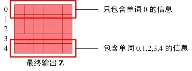
5.3 Softmax预测输出单词
Decoder block最后的部分是利用Softmax预测下一个单词,在之前的网络层我们可以得到一个最终的输出 Z Z Z,因为Mask的存在,使得单词0的输出 Z 0 Z0 Z0只包含单词0的信息,如下:
Softmax根据输出矩阵的每一行预测下一个单词:
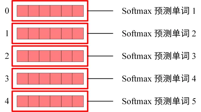
这就是Decoder block的定义,与Encoder一样,Decoder是由多个Decoder block组合而成。
二、Japanese-Chinese Machine Translation Model with Transformer & PyTorch
A tutorial using Jupyter Notebook, PyTorch, Torchtext, and SentencePiece
2.1 Import required packages
Firstly, let’s make sure we have the below packages installed in our system, if you found that some packages are missing, make sure to install them.
!pip install torchtext==0.6.0
!pip install torch
!pip install sentencepiece==0.2.0
!pip install tqdm
!pip install pandas
!pip install numpy
import math
import torchtext
import torch
import torch.nn as nn
from torch import Tensor
from torch.nn.utils.rnn import pad_sequence
from torch.utils.data import DataLoader
from collections import Counter
from torchtext.vocab import Vocab
from torch.nn import TransformerEncoder, TransformerDecoder, TransformerEncoderLayer, TransformerDecoderLayer
import io
import time
import pandas as pd
import numpy as np
import pickle
import tqdm
import sentencepiece as spm
torch.manual_seed(0)
device = torch.device('cuda' if torch.cuda.is_available() else 'cpu')
# print(torch.cuda.get_device_name(0)) ## 如果你有GPU,请在你自己的电脑上尝试运行这一套代码
device
device(type='cuda')
2.2 Get the parallel dataset
In this tutorial, we will use the Japanese-English parallel dataset downloaded from JParaCrawl![http://www.kecl.ntt.co.jp/icl/lirg/jparacrawl] which is described as the “largest publicly available English-Japanese parallel corpus created by NTT. It was created by largely crawling the web and automatically aligning parallel sentences.” You can also see the paper here.
df = pd.read_csv('./zh-ja/zh-ja.bicleaner05.txt', sep='\\t', engine='python', header=None)
trainen = df[2].values.tolist()#[:10000]
trainja = df[3].values.tolist()#[:10000]
# trainen.pop(5972)
# trainja.pop(5972)
After importing all the Japanese and their English counterparts, I deleted the last data in the dataset because it has a missing value. In total, the number of sentences in both trainen and trainja is 5,973,071, however, for learning purposes, it is often recommended to sample the data and make sure everything is working as intended, before using all the data at once, to save time.
Here is an example of sentence contained in the dataset.
print(trainen[500])
print(trainja[500])
Chinese HS Code Harmonized Code System < HS编码 2905 无环醇及其卤化、磺化、硝化或亚硝化衍生物 HS Code List (Harmonized System Code) for US, UK, EU, China, India, France, Japan, Russia, Germany, Korea, Canada ...
Japanese HS Code Harmonized Code System < HSコード 2905 非環式アルコール並びにそのハロゲン化誘導体、スルホン化誘導体、ニトロ化誘導体及びニトロソ化誘導体 HS Code List (Harmonized System Code) for US, UK, EU, China, India, France, Japan, Russia, Germany, Korea, Canada ...
We can also use different parallel datasets to follow along with this article, just make sure that we can process the data into the two lists of strings as shown above, containing the Japanese and English sentences.
2.3 Prepare the tokenizers
Unlike English or other alphabetical languages, a Japanese sentence does not contain whitespaces to separate the words. We can use the tokenizers provided by JParaCrawl which was created using SentencePiece for both Japanese and English, you can visit the JParaCrawl website to download them, or click here.
en_tokenizer = spm.SentencePieceProcessor(model_file='enja_spm_models/spm.en.nopretok.model')
ja_tokenizer = spm.SentencePieceProcessor(model_file='enja_spm_models/spm.ja.nopretok.model')
After the tokenizers are loaded, you can test them, for example, by executing the below code.
en_tokenizer.encode("All residents aged 20 to 59 years who live in Japan must enroll in public pension system.")
[227,
 2980,
 8863,
 373,
 8,
 9381,
 126,
 91,
 649,
 11,
 93,
 240,
 19228,
 11,
 419,
 14926,
 102,
 5]
ja_tokenizer.encode("年金 日本に住んでいる20歳~60歳の全ての人は、公的年金制度に加入しなければなりません。")
[4,
 31,
 346,
 912,
 10050,
 222,
 1337,
 372,
 820,
 4559,
 858,
 750,
 3,
 13118,
 31,
 346,
 2000,
 10,
 8978,
 5461,
 5]
2.4 Build the TorchText Vocab objects and convert the sentences into Torch tensors
Using the tokenizers and raw sentences, we then build the Vocab object imported from TorchText. This process can take a few seconds or minutes depending on the size of our dataset and computing power. Different tokenizer can also affect the time needed to build the vocab, I tried several other tokenizers for Japanese but SentencePiece seems to be working well and fast enough for me.
def build_vocab(sentences, tokenizer):
  counter = Counter()
  for sentence in sentences:
    counter.update(tokenizer.encode(sentence))
  return Vocab(counter, specials=['<unk>', '<pad>', '<bos>', '<eos>'])
ja_vocab = build_vocab(trainja, ja_tokenizer)
en_vocab = build_vocab(trainen, en_tokenizer)
After we have the vocabulary objects, we can then use the vocab and the tokenizer objects to build the tensors for our training data.
def data_process(ja, en):
  data = []
  for (raw_ja, raw_en) in zip(ja, en):
    ja_tensor_ = torch.tensor([ja_vocab[token] for token in ja_tokenizer.encode(raw_ja.rstrip("\n"))],
                            dtype=torch.long)
    en_tensor_ = torch.tensor([en_vocab[token] for token in en_tokenizer.encode(raw_en.rstrip("\n"))],
                            dtype=torch.long)
    data.append((ja_tensor_, en_tensor_))
  return data
train_data = data_process(trainja, trainen)
2.5 Create the DataLoader object to be iterated during training
Here, I set the BATCH_SIZE to 16 to prevent “cuda out of memory”, but this depends on various things such as your machine memory capacity, size of data, etc., so feel free to change the batch size according to your needs (note: the tutorial from PyTorch sets the batch size as 128 using the Multi30k German-English dataset.)
BATCH_SIZE = 8
PAD_IDX = ja_vocab['<pad>']
BOS_IDX = ja_vocab['<bos>']
EOS_IDX = ja_vocab['<eos>']
def generate_batch(data_batch):
  ja_batch, en_batch = [], []
  for (ja_item, en_item) in data_batch:
    ja_batch.append(torch.cat([torch.tensor([BOS_IDX]), ja_item, torch.tensor([EOS_IDX])], dim=0))
    en_batch.append(torch.cat([torch.tensor([BOS_IDX]), en_item, torch.tensor([EOS_IDX])], dim=0))
  ja_batch = pad_sequence(ja_batch, padding_value=PAD_IDX)
  en_batch = pad_sequence(en_batch, padding_value=PAD_IDX)
  return ja_batch, en_batch
train_iter = DataLoader(train_data, batch_size=BATCH_SIZE,
                        shuffle=True, collate_fn=generate_batch)
2.6 Sequence-to-sequence Transformer
The next couple of codes and text explanations (written in italic) are taken from the original PyTorch tutorial [https://pytorch.org/tutorials/beginner/translation_transformer.html]. I did not make any change except for the BATCH_SIZE and the word de_vocabwhich is changed to ja_vocab.
Transformer is a Seq2Seq model introduced in “Attention is all you need” paper for solving machine translation task. Transformer model consists of an encoder and decoder block each containing fixed number of layers.
Encoder processes the input sequence by propagating it, through a series of Multi-head Attention and Feed forward network layers. The output from the Encoder referred to as memory, is fed to the decoder along with target tensors. Encoder and decoder are trained in an end-to-end fashion using teacher forcing technique.
from torch.nn import (TransformerEncoder, TransformerDecoder,
                      TransformerEncoderLayer, TransformerDecoderLayer)


class Seq2SeqTransformer(nn.Module):
    def __init__(self, num_encoder_layers: int, num_decoder_layers: int,
                 emb_size: int, src_vocab_size: int, tgt_vocab_size: int,
                 dim_feedforward:int = 512, dropout:float = 0.1):
        super(Seq2SeqTransformer, self).__init__()
        encoder_layer = TransformerEncoderLayer(d_model=emb_size, nhead=NHEAD,
                                                dim_feedforward=dim_feedforward)
        self.transformer_encoder = TransformerEncoder(encoder_layer, num_layers=num_encoder_layers)
        decoder_layer = TransformerDecoderLayer(d_model=emb_size, nhead=NHEAD,
                                                dim_feedforward=dim_feedforward)
        self.transformer_decoder = TransformerDecoder(decoder_layer, num_layers=num_decoder_layers)

        self.generator = nn.Linear(emb_size, tgt_vocab_size)
        self.src_tok_emb = TokenEmbedding(src_vocab_size, emb_size)
        self.tgt_tok_emb = TokenEmbedding(tgt_vocab_size, emb_size)
        self.positional_encoding = PositionalEncoding(emb_size, dropout=dropout)

    def forward(self, src: Tensor, trg: Tensor, src_mask: Tensor,
                tgt_mask: Tensor, src_padding_mask: Tensor,
                tgt_padding_mask: Tensor, memory_key_padding_mask: Tensor):
        src_emb = self.positional_encoding(self.src_tok_emb(src))
        tgt_emb = self.positional_encoding(self.tgt_tok_emb(trg))
        memory = self.transformer_encoder(src_emb, src_mask, src_padding_mask)
        outs = self.transformer_decoder(tgt_emb, memory, tgt_mask, None,
                                        tgt_padding_mask, memory_key_padding_mask)
        return self.generator(outs)

    def encode(self, src: Tensor, src_mask: Tensor):
        return self.transformer_encoder(self.positional_encoding(
                            self.src_tok_emb(src)), src_mask)

    def decode(self, tgt: Tensor, memory: Tensor, tgt_mask: Tensor):
        return self.transformer_decoder(self.positional_encoding(
                          self.tgt_tok_emb(tgt)), memory,
                          tgt_mask)
Text tokens are represented by using token embeddings. Positional encoding is added to the token embedding to introduce a notion of word order.
class PositionalEncoding(nn.Module):
    def __init__(self, emb_size: int, dropout, maxlen: int = 5000):
        super(PositionalEncoding, self).__init__()
        den = torch.exp(- torch.arange(0, emb_size, 2) * math.log(10000) / emb_size)
        pos = torch.arange(0, maxlen).reshape(maxlen, 1)
        pos_embedding = torch.zeros((maxlen, emb_size))
        pos_embedding[:, 0::2] = torch.sin(pos * den)
        pos_embedding[:, 1::2] = torch.cos(pos * den)
        pos_embedding = pos_embedding.unsqueeze(-2)

        self.dropout = nn.Dropout(dropout)
        self.register_buffer('pos_embedding', pos_embedding)

    def forward(self, token_embedding: Tensor):
        return self.dropout(token_embedding +
                            self.pos_embedding[:token_embedding.size(0),:])

class TokenEmbedding(nn.Module):
    def __init__(self, vocab_size: int, emb_size):
        super(TokenEmbedding, self).__init__()
        self.embedding = nn.Embedding(vocab_size, emb_size)
        self.emb_size = emb_size
    def forward(self, tokens: Tensor):
        return self.embedding(tokens.long()) * math.sqrt(self.emb_size)
We create a subsequent word mask to stop a target word from attending to its subsequent words. We also create masks, for masking source and target padding tokens
def generate_square_subsequent_mask(sz):
    mask = (torch.triu(torch.ones((sz, sz), device=device)) == 1).transpose(0, 1)
    mask = mask.float().masked_fill(mask == 0, float('-inf')).masked_fill(mask == 1, float(0.0))
    return mask

def create_mask(src, tgt):
  src_seq_len = src.shape[0]
  tgt_seq_len = tgt.shape[0]

  tgt_mask = generate_square_subsequent_mask(tgt_seq_len)
  src_mask = torch.zeros((src_seq_len, src_seq_len), device=device).type(torch.bool)

  src_padding_mask = (src == PAD_IDX).transpose(0, 1)
  tgt_padding_mask = (tgt == PAD_IDX).transpose(0, 1)
  return src_mask, tgt_mask, src_padding_mask, tgt_padding_mask
Define model parameters and instantiate model. 这里我们服务器实在是计算能力有限,按照以下配置可以训练但是效果应该是不行的。如果想要看到训练的效果请使用你自己的带GPU的电脑运行这一套代码。
当你使用自己的GPU的时候,NUM_ENCODER_LAYERS 和 NUM_DECODER_LAYERS 设置为3或者更高,NHEAD设置8,EMB_SIZE设置为512。
SRC_VOCAB_SIZE = len(ja_vocab)
TGT_VOCAB_SIZE = len(en_vocab)
EMB_SIZE = 512
NHEAD = 8
FFN_HID_DIM = 512
BATCH_SIZE = 16
NUM_ENCODER_LAYERS = 3
NUM_DECODER_LAYERS = 3
NUM_EPOCHS = 16
transformer = Seq2SeqTransformer(NUM_ENCODER_LAYERS, NUM_DECODER_LAYERS,
                                 EMB_SIZE, SRC_VOCAB_SIZE, TGT_VOCAB_SIZE,
                                 FFN_HID_DIM)

for p in transformer.parameters():
    if p.dim() > 1:
        nn.init.xavier_uniform_(p)

transformer = transformer.to(device)

loss_fn = torch.nn.CrossEntropyLoss(ignore_index=PAD_IDX)

optimizer = torch.optim.Adam(
    transformer.parameters(), lr=0.0001, betas=(0.9, 0.98), eps=1e-9
)
def train_epoch(model, train_iter, optimizer):
  model.train()
  losses = 0
  for idx, (src, tgt) in  enumerate(train_iter):
      src = src.to(device)
      tgt = tgt.to(device)

      tgt_input = tgt[:-1, :]

      src_mask, tgt_mask, src_padding_mask, tgt_padding_mask = create_mask(src, tgt_input)

      logits = model(src, tgt_input, src_mask, tgt_mask,
                                src_padding_mask, tgt_padding_mask, src_padding_mask)

      optimizer.zero_grad()

      tgt_out = tgt[1:,:]
      loss = loss_fn(logits.reshape(-1, logits.shape[-1]), tgt_out.reshape(-1))
      loss.backward()

      optimizer.step()
      losses += loss.item()
  return losses / len(train_iter)


def evaluate(model, val_iter):
  model.eval()
  losses = 0
  for idx, (src, tgt) in (enumerate(valid_iter)):
    src = src.to(device)
    tgt = tgt.to(device)

    tgt_input = tgt[:-1, :]

    src_mask, tgt_mask, src_padding_mask, tgt_padding_mask = create_mask(src, tgt_input)

    logits = model(src, tgt_input, src_mask, tgt_mask,
                              src_padding_mask, tgt_padding_mask, src_padding_mask)
    tgt_out = tgt[1:,:]
    loss = loss_fn(logits.reshape(-1, logits.shape[-1]), tgt_out.reshape(-1))
    losses += loss.item()
  return losses / len(val_iter)
2.7 Start training
Finally, after preparing the necessary classes and functions, we are ready to train our model. This goes without saying but the time needed to finish training could vary greatly depending on a lot of things such as computing power, parameters, and size of datasets.
When I trained the model using the complete list of sentences from JParaCrawl which has around 5.9 million sentences for each language, it took around 5 hours per epoch using a single NVIDIA GeForce RTX 3070 GPU.
Here is the code:
for epoch in tqdm.tqdm(range(1, NUM_EPOCHS+1)):
  start_time = time.time()
  train_loss = train_epoch(transformer, train_iter, optimizer)
  end_time = time.time()
  print((f"Epoch: {epoch}, Train loss: {train_loss:.3f}, "
          f"Epoch time = {(end_time - start_time):.3f}s"))
  6%|▋         | 1/16 [03:11<47:46, 191.12s/it]

Epoch: 1, Train loss: 4.438, Epoch time = 191.117s


 12%|█▎        | 2/16 [06:11<43:04, 184.60s/it]

Epoch: 2, Train loss: 3.462, Epoch time = 180.038s


 19%|█▉        | 3/16 [09:14<39:52, 184.03s/it]

Epoch: 3, Train loss: 3.054, Epoch time = 183.344s


 25%|██▌       | 4/16 [12:29<37:40, 188.37s/it]

Epoch: 4, Train loss: 2.756, Epoch time = 195.019s


 31%|███▏      | 5/16 [15:43<34:53, 190.32s/it]

Epoch: 5, Train loss: 2.536, Epoch time = 193.788s


 38%|███▊      | 6/16 [18:47<31:23, 188.37s/it]

Epoch: 6, Train loss: 2.368, Epoch time = 184.564s


 44%|████▍     | 7/16 [21:51<27:59, 186.66s/it]

Epoch: 7, Train loss: 2.263, Epoch time = 183.150s


 50%|█████     | 8/16 [24:51<24:37, 184.69s/it]

Epoch: 8, Train loss: 2.167, Epoch time = 180.480s


 56%|█████▋    | 9/16 [27:51<21:22, 183.20s/it]

Epoch: 9, Train loss: 2.085, Epoch time = 179.901s


 62%|██████▎   | 10/16 [30:52<18:14, 182.43s/it]

Epoch: 10, Train loss: 2.014, Epoch time = 180.713s


 69%|██████▉   | 11/16 [33:53<15:09, 181.98s/it]

Epoch: 11, Train loss: 1.955, Epoch time = 180.954s


 75%|███████▌  | 12/16 [36:51<12:03, 180.99s/it]

Epoch: 12, Train loss: 1.901, Epoch time = 178.734s


 81%|████████▏ | 13/16 [39:52<09:02, 180.77s/it]

Epoch: 13, Train loss: 1.854, Epoch time = 180.264s


 88%|████████▊ | 14/16 [42:51<06:00, 180.22s/it]

Epoch: 14, Train loss: 1.813, Epoch time = 178.936s


 94%|█████████▍| 15/16 [46:01<03:03, 183.30s/it]

Epoch: 15, Train loss: 1.776, Epoch time = 190.444s


100%|██████████| 16/16 [49:00<00:00, 183.77s/it]

Epoch: 16, Train loss: 1.739, Epoch time = 178.832s
2.8 Try translating a Japanese sentence using the trained model
First, we create the functions to translate a new sentence, including steps such as to get the Japanese sentence, tokenize, convert to tensors, inference, and then decode the result back into a sentence, but this time in English.
def greedy_decode(model, src, src_mask, max_len, start_symbol):
    src = src.to(device)
    src_mask = src_mask.to(device)
    memory = model.encode(src, src_mask)
    ys = torch.ones(1, 1).fill_(start_symbol).type(torch.long).to(device)
    for i in range(max_len-1):
        memory = memory.to(device)
        memory_mask = torch.zeros(ys.shape[0], memory.shape[0]).to(device).type(torch.bool)
        tgt_mask = (generate_square_subsequent_mask(ys.size(0))
                                    .type(torch.bool)).to(device)
        out = model.decode(ys, memory, tgt_mask)
        out = out.transpose(0, 1)
        prob = model.generator(out[:, -1])
        _, next_word = torch.max(prob, dim = 1)
        next_word = next_word.item()
        ys = torch.cat([ys,
                        torch.ones(1, 1).type_as(src.data).fill_(next_word)], dim=0)
        if next_word == EOS_IDX:
          break
    return ys
def translate(model, src, src_vocab, tgt_vocab, src_tokenizer):
    model.eval()
    tokens = [BOS_IDX] + [src_vocab.stoi[tok] for tok in src_tokenizer.encode(src, out_type=str)]+ [EOS_IDX]
    num_tokens = len(tokens)
    src = (torch.LongTensor(tokens).reshape(num_tokens, 1) )
    src_mask = (torch.zeros(num_tokens, num_tokens)).type(torch.bool)
    tgt_tokens = greedy_decode(model,  src, src_mask, max_len=num_tokens + 5, start_symbol=BOS_IDX).flatten()
    print(tgt_vocab)
    Str=" ".join([str((tgt_vocab).itos[tok]) for tok in tgt_tokens]).replace("<bos>", "").replace("<eos>", "")
    return " ".join([str((tgt_vocab).itos[tok]) for tok in tgt_tokens]).replace("<bos>", "").replace("<eos>", "")
Then, we can just call the translate function and pass the required parameters.
translate(transformer, "HSコード 8515 はんだ付け用、ろう付け用又は溶接用の機器(電気式(電気加熱ガス式を含む。)", ja_vocab, en_vocab, ja_tokenizer)
<torchtext.vocab.Vocab object at 0x7fd255670c40>

' 41 24981 25304 24647 26946 24647 26946 24647 26946 24647 26946 24647 26946 24647 24502 41 25117 26856 25823 23506 25117 41 25117 24401 25117 24401 25117 24401 41 25117 24401 41 25117 24401 41 25117'
trainen.pop(5)
'Chinese HS Code Harmonized Code System < HS编码 8515 : 电气(包括电热气体)、激光、其他光、光子束、超声波、电子束、磁脉冲或等离子弧焊接机器及装置,不论是否 HS Code List (Harmonized System Code) for US, UK, EU, China, India, France, Japan, Russia, Germany, Korea, Canada ...'
trainja.pop(5)
'Japanese HS Code Harmonized Code System < HSコード 8515 はんだ付け用、ろう付け用又は溶接用の機器(電気式(電気加熱ガス式を含む。)、レーザーその他の光子ビーム式、超音波式、電子ビーム式、 HS Code List (Harmonized System Code) for US, UK, EU, China, India, France, Japan, Russia, Germany, Korea, Canada ...'
2.9 Save the Vocab objects and trained model
Finally, after the training has finished, we will save the Vocab objects (en_vocab and ja_vocab) first, using Pickle.
import pickle
# open a file, where you want to store the data
file = open('en_vocab.pkl', 'wb')
# dump information to that file
pickle.dump(en_vocab, file)
file.close()
file = open('ja_vocab.pkl', 'wb')
pickle.dump(ja_vocab, file)
file.close()
Lastly, we can also save the model for later use using PyTorch save and load functions. Generally, there are two ways to save the model depending what we want to use them for later. The first one is for inference only, we can load the model later and use it to translate from Japanese to English.
# save model for inference
torch.save(transformer.state_dict(), 'inference_model')
The second one is for inference too, but also for when we want to load the model later, and want to resume the training.
# save model + checkpoint to resume training later
torch.save({
  'epoch': NUM_EPOCHS,
  'model_state_dict': transformer.state_dict(),
  'optimizer_state_dict': optimizer.state_dict(),
  'loss': train_loss,
  }, 'model_checkpoint.tar')
三、实验总结
- Transformer与RNN不同,可以比较好地并行训练。
- Transformer本身是不能利用单词的顺序信息的,因此需要在输入中添加位置Embedding,否则 Transformer就是一个词袋模型了。
- Transformer的重点是Self-Attention 结构,其中用到的 Q , K , V Q, K, V Q,K,V矩阵通过输出进行线性变换得到。
- Transformer中Multi-Head Attention中有多个Self-Attention,可以捕获单词之间多种维度上的相关系数attention score。
四、参考文献
[1] 实验14.基于Transformer实现机器翻译(日译中)(有GPU的同学需运行出来,没有GPU的同学需看懂代码适当注释) (educg.net)
[2] 深度解析 Transformer 模型:原理、应用与实践指南【收藏版】_自注意力机制的计算过程包括三个步骤:计算注意力权重、将加权的位置向量作为输出-CSDN博客


 被折叠的 条评论
为什么被折叠?
被折叠的 条评论
为什么被折叠?
 到【灌水乐园】发言


