西瓜书3.3对率回归

西瓜书3.3

这是西瓜书第一道实践题，感觉书里对于原理讲解过于生硬，有点难以理解，所以我更多采用从andrew ng的深度学习中学到的logistic regression来描述

对率回归西瓜数据3.0alpha

数据如下

编号	密度	糖分	好瓜
0	0.697	0.460	1
1	0.774	0.376	1
2	0.634	0.264	1
3	0.608	0.318	1
4	0.556	0.215	1
5	0.403	0.237	1
6	0.481	0.149	1
7	0.437	0.211	1
8	0.666	0.091	0
9	0.243	0.267	0
10	0.245	0.057	0
11	0.343	0.099	0
12	0.639	0.161	0
13	0.657	0.198	0
14	0.360	0.370	0
15	0.593	0.042	0
16	0.719	0.103	0

导入数据

import pandas as pd
import numpy as np
from sklearn.model_selection import train_test_split

df = pd.DataFrame({'midu':[0.697,0.774,0.634,0.608,0.556,0.403,0.481,0.437, 0.666,0.243,0.245,0.343,0.639,0.657,0.360,0.593,0.719],
                   'tang':[0.460,0.376,0.264,0.318,0.215,0.237,0.149,0.211, 0.091,0.267,0.057,0.099,0.161,0.198,0.370,0.042,0.103],
                   'hao': [1,1,1,1,1,1,1,1, 0,0,0,0,0,0,0,0,0]})
X = df[['midu','tang']].values
y = df['hao'].values
#为了使数据形式符合需要演示需要，将其进行转置
X = X.reshape([2,17])
y = y.reshape([1,17])

参数的随机生成和sigmoid激活函数定义

'''
initialize parameter
'''
def init_params():
	#根据X数据的形状来确定生成w和b
    w = np.random.randn(2, 1)
    b = 0
    return w, b
'''
sigmoid activation func
'''
def sigmoid(Z):
    s = 1 / (1+np.exp(-Z))
    return s

传播和参数优化（gradient descent）

向前传播:

• You get X
• $A=\sigma (w^{T}X+b)=(a^{(1)},a^{(2)},...,a^{(m-1)},a^{(m)})$
• cost function:
• $J=-\frac{1}{m}{\sum }_{i=1}^m{y}^{(i)}\log (a^{(i)})+(1-y^{(i)})\log (1-a^{(i)})$

由cost func对w 和b分别求导:

$$\frac{\partial J}{\partial w}=\frac{1}{m}X(A-Y{)}^T\text{\hspace{1em}(7)}$$
$$\frac{\partial J}{\partial b}=\frac{1}{m}\sum _{i=1}^m(a^{(i)}-y^{(i)})\text{\hspace{1em}(8)}$$

'''
forward prop and compute cost and back prop
'''
def f_prop(w, b, X, y):
    m = X.shape[1]#一共有m个实例
    A = sigmoid(np.dot(w.T, X) + b)
    #计算cost函数
    cost = -1/m * np.sum(y*np.log(A) + (1-y)*np.log(1-A))
    #对w和b求导数
    dw = 1/m * np.dot(X, (A-y).T)
    db = 1/m * np.sum(A - y)
    #组合到一个字典
    grads = {'dw':dw, 'db':db}
    return cost, grads
'''
optimize parameters--gradient descent
'''
def op_params(w, b, X, y, num_iter, learning_rate):
    costs = []
    
    for i in range(num_iter):
        cost ,grads = f_prop(w, b, X, y)
        dw = grads['dw']
        db = grads['db']
        #参数最优化
        w = w - learning_rate * dw
        b = b - learning_rate * db
        costs.append(cost)
    
    params = {'w':w, 'b':b}

    return costs, params    

预测函数

'''
predict
'''
def predict(params, X):
    m = X.shape[1]
    Y_prediction = np.zeros((1,m))
    
    w = params['w']
    b = params['b']
    A = sigmoid(np.dot(w.T, X)+b) 
    #大于0.5就是真，小于等于0.5就是假
    for i in range(m):
        if A[0, i] > 0.5:
            Y_prediction[0, i] = 1
        if A[0, i] <= 0.5:
            Y_prediction[0, i] = 0
    return Y_prediction

模型建立和参数获取

%matplotlib notebook 
import matplotlib.pyplot as plt
'''
merge all the func
'''
w, b = init_params()
cost, grads = f_prop(w, b, X, y)
costs, params = op_params(w, b, X, y, 1000, 0.9)
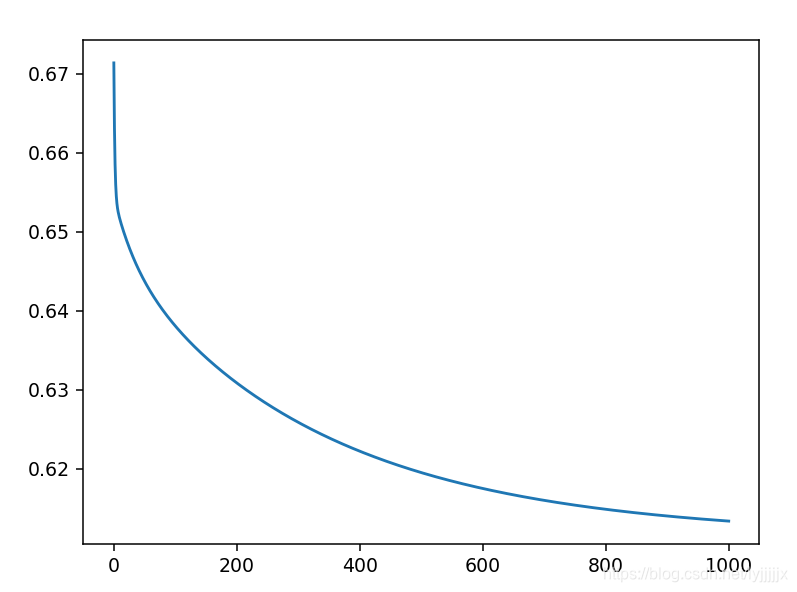
plt.plot(costs)

最后的损失函数曲线，1000次循环， 0.9学习率:

训练集预测

'''
make prediction
'''
Y_prediction = predict(params, X)

count = 0
for i in range(X.shape[1]):
    if Y_perdiction[0, i] == y[0, i]:
        count += 1

precision = count/X.shape[1]
print('准确率是：',precision)

准确率是： 0.5882352941176471
显然，这个模型使underfit的，但是基于有限的数据集，且cost func已经达到极限，所以很难再找到更优的参数，就先这样吧。