Python学习---scikit-learn 0.23公布的亮点

Generalized Linear Models, and Poisson loss for gradient boosting¶
Long-awaited Generalized Linear Models with non-normal loss functions
are now available. In particular, three new regressors were
implemented: PoissonRegressor, GammaRegressor, and TweedieRegressor.
The Poisson regressor can be used to model positive integer counts, or
relative frequencies. Read more in the User Guide. Additionally,
HistGradientBoostingRegressor supports a new ‘poisson’ loss as well.

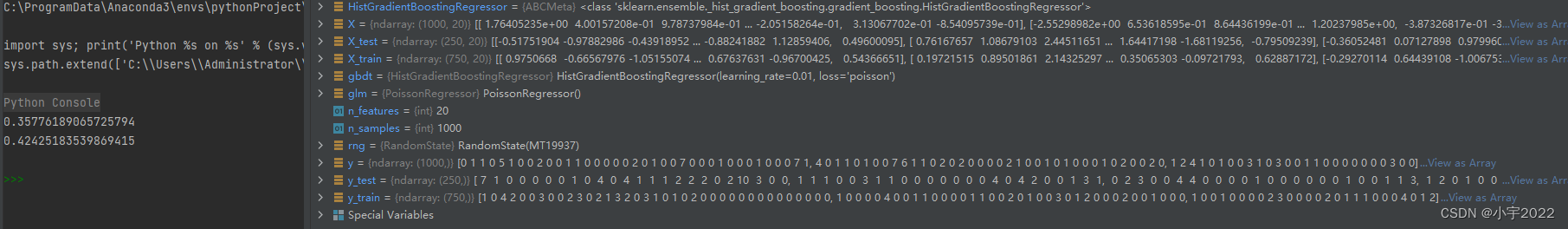
import numpy as np
from sklearn.model_selection import train_test_split
from sklearn.linear_model import PoissonRegressor
from sklearn.ensemble import HistGradientBoostingRegressor

n_samples, n_features = 1000, 20
rng = np.random.RandomState(0)
X = rng.randn(n_samples, n_features)
# positive integer target correlated with X[:, 5] with many zeros:
y = rng.poisson(lam=np.exp(X[:, 5]) / 2)
X_train, X_test, y_train, y_test = train_test_split(X, y, random_state=rng)
glm = PoissonRegressor()
gbdt = HistGradientBoostingRegressor(loss="poisson", learning_rate=0.01)
glm.fit(X_train, y_train)
gbdt.fit(X_train, y_train)
print(glm.score(X_test, y_test))
print(gbdt.score(X_test, y_test))

Scalability and stability improvements to KMeans¶ The KMeans estimator
was entirely re-worked, and it is now significantly faster and more
stable. In addition, the Elkan algorithm is now compatible with sparse
matrices. The estimator uses OpenMP based parallelism instead of
relying on joblib, so the n_jobs parameter has no effect anymore. For
more details on how to control the number of threads, please refer to
our Parallelism notes.

import scipy
import numpy as np
from sklearn.model_selection import train_test_split
from sklearn.cluster import KMeans
from sklearn.datasets import make_blobs
from sklearn.metrics import completeness_score

rng = np.random.RandomState(0)
X, y = make_blobs(random_state=rng)
X = scipy.sparse.csr_matrix(X)
X_train, X_test, _, y_test = train_test_split(X, y, random_state=rng)
kmeans = KMeans(algorithm="elkan").fit(X_train)
print(completeness_score(kmeans.predict(X_test), y_test))

Improvements to the histogram-based Gradient Boosting estimators
Various improvements were made to HistGradientBoostingClassifier and
HistGradientBoostingRegressor. On top of the Poisson loss mentioned
above, these estimators now support sample weights. Also, an automatic
early-stopping criterion was added: early-stopping is enabled by
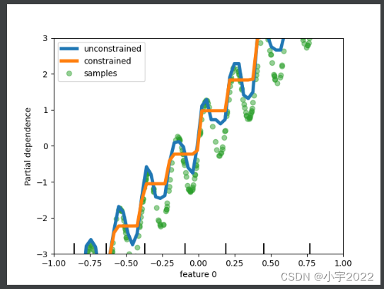
default when the number of samples exceeds 10k. Finally, users can now
define monotonic constraints to constrain the predictions based on the
variations of specific features. In the following example, we
construct a target that is generally positively correlated with the
first feature, with some noise. Applying monotoinc constraints allows
the prediction to capture the global effect of the first feature,
instead of fitting the noise.

import numpy as np
from matplotlib import pyplot as plt
from sklearn.model_selection import train_test_split
from sklearn.inspection import plot_partial_dependence
from sklearn.ensemble import HistGradientBoostingRegressor

n_samples = 500
rng = np.random.RandomState(0)
X = rng.randn(n_samples, 2)
noise = rng.normal(loc=0.0, scale=0.01, size=n_samples)
y = 5 * X[:, 0] + np.sin(10 * np.pi * X[:, 0]) - noise

gbdt_no_cst = HistGradientBoostingRegressor().fit(X, y)
gbdt_cst = HistGradientBoostingRegressor(monotonic_cst=[1, 0]).fit(X, y)

disp = plot_partial_dependence(
    gbdt_no_cst,
    X,
    features=[0],
    feature_names=["feature 0"],
    line_kw={"linewidth": 4, "label": "unconstrained", "color": "tab:blue"},
)
plot_partial_dependence(
    gbdt_cst,
    X,
    features=[0],
    line_kw={"linewidth": 4, "label": "constrained", "color": "tab:orange"},
    ax=disp.axes_,
)
disp.axes_[0, 0].plot(
    X[:, 0], y, "o", alpha=0.5, zorder=-1, label="samples", color="tab:green"
)
disp.axes_[0, 0].set_ylim(-3, 3)
disp.axes_[0, 0].set_xlim(-1, 1)
plt.legend()
plt.show()

Release Highlights for scikit-learn 0.23