机器学习之逻辑回归

一、逻辑回归基本介绍

Logistic Regression

1. 用于分类问题
2. 监督学习算法

---

二、逻辑回归工作原理

根据现有数据对分类边界线建立回归公式 ，具体分为以下三步

1. 将决策边界表示为

z = W₁X₁+W₂X₂+···+W_nX_n + b (W₀X₀)

向量x是分类器的输入数据，向量θ是我们要找到的最佳参数。

2. 把决策边界函数经过Sigmoid函数运算得到概率：

• 概率大于0.5分类为1
• 概率小于0.5分类为0

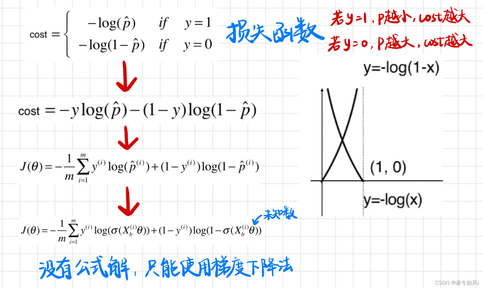
3.使损失函数最小化来获得最佳的参数向量θ

如果分类为1，则概率越小表示分类错误程度越高；如果分类为0，则概率越大表示分类错误程度越高。经过推导，最后用梯度下降法计算损失函数最小值。

---

三、python实现逻辑回归

import random

import numpy as np
import matplotlib.pyplot as plt

def loadDataSet():
    dataMat = []
    labelMat = []
    f = open("testSet.txt")
    for line in f.readlines():
        lineArr = line.strip().split()
        dataMat.append([1.0, float(lineArr[0]), float(lineArr[1])])
        labelMat.append(int(lineArr[2]))
    f.close()
    return dataMat, labelMat


def sigmoid(inX):
    return 1.0/(1+np.exp(-inX))


"""
这里的损失函数简单使用：
1-p if y=1
p if y=0
损失函数=|正确值y - 预测值p|
符合如果y=1 p越小,cost越大, 如果y=0,p越大,cost越大
"""
def gradAscent(dataMatIn, classLabels):
    dataMatrix = np.mat(dataMatIn)  # 转换成np的mat格式
    labelMatrix = np.mat(classLabels).transpose()  # 转换成np的mat格式并进行转置
    m, n = np.shape(dataMatrix)
    alpha = 0.001    # 学习率
    maxCycles = 500  # 最大迭代次数
    weights = np.ones((n, 1))  # 创建一个n行1列的数组，每个回归系数初始化为1,loadDataSet()已经将X0设为1;   WX = w0(X0=1) + w1X1 + w2X2
    for k in range(maxCycles):
        h = sigmoid(dataMatrix*weights)
        error = (labelMatrix - h)                               # 对函数关于回归系数求导后得到参数更新的表达式：w = w +α(h-y)x
        weights = weights + alpha*dataMatrix.transpose()*error  # 定性地说，此处计算真实类别与预测类别的差值，接下来就是按照该差值的方向调整回归系数
    return weights.getA()   # 将矩阵转换为数组，和np.mat()相反


# 区别：1. 变量h和误差error都是数值,但在梯度下降里面是向量;
#      2. 没有矩阵转换过程,所有变量数据类型都是numpy数组
def stocGradAscent(dataMatrix, classLabels, numIter=150):
    m, n = np.shape(dataMatrix)                       # 返回dataMatrix的大小。m为行数,n为列数。
    weights = np.ones(n)                              # 参数初始化
    for j in range(numIter):
        dataIndex = list(range(m))
        for i in range(m):
            alpha = 4/(1.0+j+i)+0.01                                    # 降低alpha的大小，每次减小1/(j+i)。
            randIndex = int(random.uniform(0,len(dataIndex)))           # 随机选取样本
            h = sigmoid(sum(dataMatrix[dataIndex[randIndex]]*weights))  # 选择随机选取的一个样本，计算h
            error = classLabels[dataIndex[randIndex]] - h                          # 计算误差
            weights = weights + alpha * error * dataMatrix[dataIndex[randIndex]]   # 更新回归系数
            del(dataIndex[randIndex])                                         # 删除已经使用的样本
    return weights


def plotBestFit(weights):
    dataMat, labelMat = loadDataSet()  # 加载数据集
    dataArr = np.array(dataMat)  # 转换成numpy的array数组
    n = np.shape(dataMat)[0]  # 数据个数
    xcord1 = []; ycord1 = []  # 正样本
    xcord2 = []; ycord2 = []  # 负样本
    for i in range(n):  # 根据数据集标签进行分类
        if int(labelMat[i]) == 1:
            xcord1.append(dataArr[i, 1]); ycord1.append(dataArr[i, 2])  # 1为正样本
        else:
            xcord2.append(dataArr[i, 1]); ycord2.append(dataArr[i, 2])  # 0为负样本
    fig = plt.figure()
    ax = fig.add_subplot(111)  # 添加subplot
    ax.scatter(xcord1, ycord1, s=20, c='red', marker='s', alpha=.5)  # 绘制正样本
    ax.scatter(xcord2, ycord2, s=20, c='green', alpha=.5)  # 绘制负样本
    x = np.arange(-3.0, 3.0, 0.1)
    y = (-weights[0] - weights[1] * x) / weights[2]
    ax.plot(x, y)
    plt.title('BestFit')  # 绘制title
    plt.xlabel('X1'); plt.ylabel('X2')  # 绘制label
    plt.show()


if __name__ == '__main__':
    dataMat, labelMat = loadDataSet()
    weights = stocGradAscent(np.array(dataMat), labelMat)
    plotBestFit(weights)

---

四、sklearn实现逻辑回归

import numpy as np
import matplotlib.pyplot as plt

np.random.seed(666)    # 设置固定的随机数种子

X = np.random.normal(0, 1, size=(200, 2))  # 均值为0,方差为1的随机数样本
y = np.array(X[:, 0]**2 + X[:, 1] < 1.5, dtype='int')  # 强制使一个Boolean类型转为int型,True则取1,False则取0

for _ in range(20):                 # 添加噪音
    y[np.random.randint(200)] = 1   # 随机挑20个点,强制让分类结果为1

plt.scatter(X[y==0, 0], X[y==0, 1])
plt.scatter(X[y==1, 0], X[y==1, 1])
plt.show()

from sklearn.model_selection import train_test_split   # 分割数据集
X_train, X_test, y_train, y_test = train_test_split(X, y, random_state=666)

# 导入LogisticRegression
from sklearn.linear_model import LogisticRegression

log_reg = LogisticRegression()
log_reg.fit(X_train, y_train)

print(log_reg.score(X_train, y_train))
print(log_reg.score(X_test, y_test))  # 分数并不高，因为样本数据是二次函数型的


# 绘制决策边界
def plot_decision_boundary(model, axis):
    x0, x1 = np.meshgrid(
        np.linspace(axis[0], axis[1], int((axis[1] - axis[0]) * 100)).reshape(-1, 1),
        np.linspace(axis[2], axis[3], int((axis[3] - axis[2]) * 100)).reshape(-1, 1),
    )
    X_new = np.c_[x0.ravel(), x1.ravel()]

    y_predict = model.predict(X_new)
    zz = y_predict.reshape(x0.shape)

    from matplotlib.colors import ListedColormap
    custom_cmap = ListedColormap(['#EF9A9A', '#FFF59D', '#90CAF9'])

    plt.contourf(x0, x1, zz, linewidth=5, cmap=custom_cmap)


plot_decision_boundary(log_reg, axis=[-4, 4, -4, 4])
plt.scatter(X[y==0,0], X[y==0,1])
plt.scatter(X[y==1,0], X[y==1,1])
plt.show()

LogisticRegression() 构造函数的参数及默认值

LogisticRegression(C=1.0, class_weight=None, dual=False, fit_intercept=True,
          intercept_scaling=1, max_iter=100, multi_class='ovr', n_jobs=1,
          penalty='l2', random_state=None, solver='liblinear', tol=0.0001,
          verbose=0, warm_start=False)

1. penalty：默认为’l2’，默认正则化方式为l2正则化，还有l1正则化。
2. C：默认是1.0，正则化参数
3. max_iter：算法收敛最大迭代次数，int类型，默认为10

sklearn中对逻辑回归进行多项式回归、正则化等

J(θ)是损失函数，L是正则化项

# 多项式回归
def PolynomialLogisticRegression(degree, C, penalty='l2'):
    return Pipeline([
        ('poly', PolynomialFeatures(degree=degree)),
        ('std_scaler', StandardScaler()),
        ('log_reg', LogisticRegression(C=C, penalty=penalty))
    ])

poly_log_reg4 = PolynomialLogisticRegression(degree=20, C=0.1, penalty='l1')
poly_log_reg4.fit(X_train, y_train)

poly_log_reg4.score(X_train, y_train)
poly_log_reg4.score(X_test, y_test)

实现多项式回归等具体内容参考bobo老师课程

---

五、决策边界的绘制

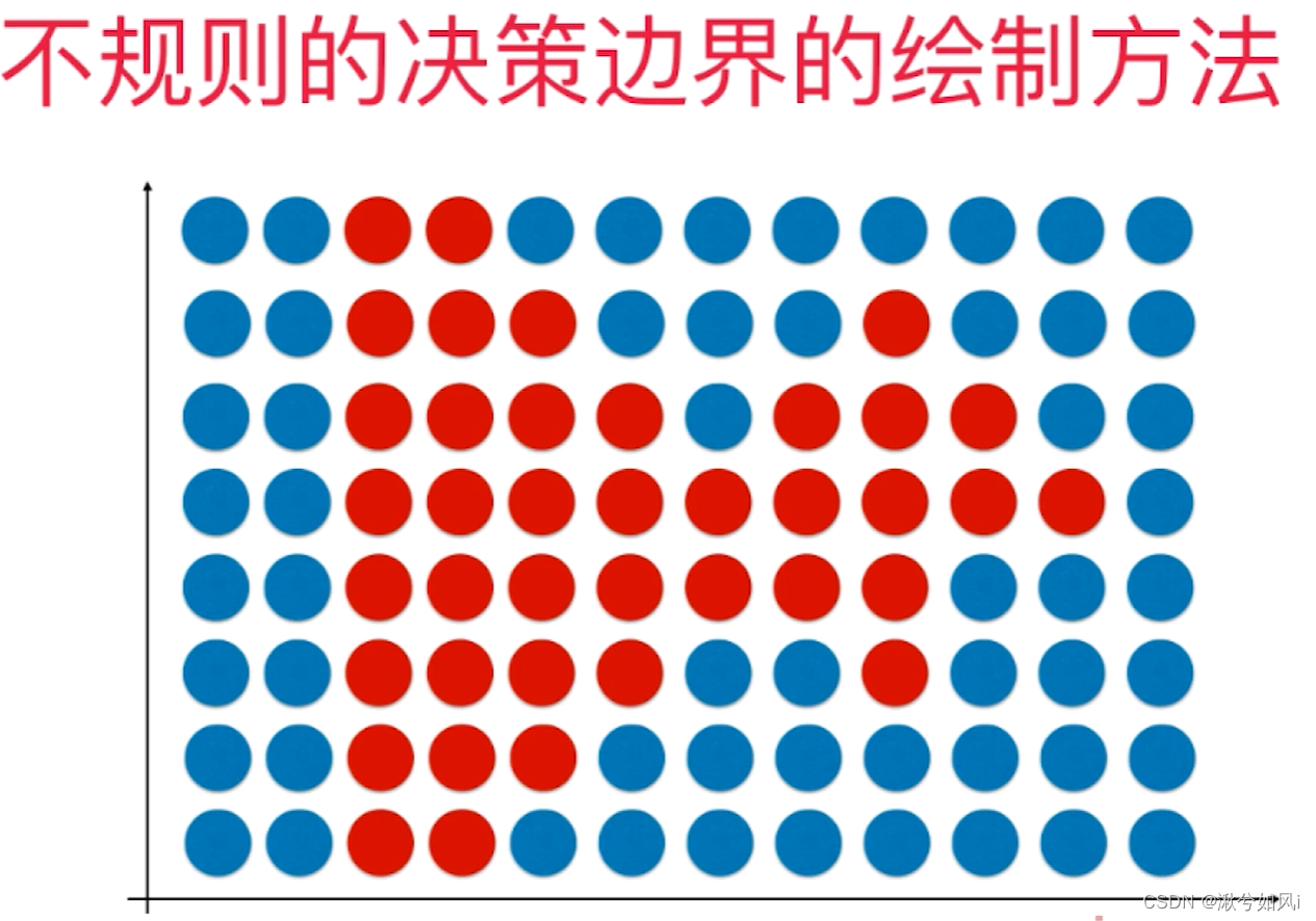
线性拟合时，我们可以通过画出决策边界线，边界上边的是一类，边界下面的是一类。但当决策边界不规则时，即不是简单的直线时，就很难用这种方法绘制出决策边界线。新的思路是：每次来一个点，判断它分为“蓝色”还是“红色”的类，对平面中足够密的点都进行判断和绘制，最后就能显现出决策边界。

# 绘制决策边界
def plot_decision_boundary(model, axis):        # axis是坐标轴的范围

    # 将x轴和y轴划分为无数的小点
    x0, x1 = np.meshgrid(
        np.linspace(axis[0], axis[1], int((axis[1] - axis[0]) * 100)).reshape(-1, 1),
        np.linspace(axis[2], axis[3], int((axis[3] - axis[2]) * 100)).reshape(-1, 1),
    )
    X_new = np.c_[x0.ravel(), x1.ravel()]   # 连接x0,x1 进行ravel扁平化

    y_predict = model.predict(X_new)     # 对于所有的点，都用model进行预测
    zz = y_predict.reshape(x0.shape)     # 扁平化后形状变了

    from matplotlib.colors import ListedColormap
    custom_cmap = ListedColormap(['#EF9A9A', '#FFF59D', '#90CAF9'])

    plt.contourf(x0, x1, zz, linewidth=5, cmap=custom_cmap)

#-----------------------------------------------------------------------------------#

plot_decision_boundary(log_reg, axis=[-4, 4, -4, 4])
plt.scatter(X[y==0,0], X[y==0,1])
plt.scatter(X[y==1,0], X[y==1,1])
plt.show()

---

总结

优缺点

1. 优点

• 训练速度较快，可解释性高

2. 缺点

• 容易欠拟合，精度不高

问题

1. 待完善