


目录
初始化
% Initialization
clear ; close all; clc
1.WarmUpExercise()
function A = warmUpExercise()

A =eye(5);

end
ex1.m
%% ==================== Part 1: Basic Function ====================
% Complete warmUpExercise.m
fprintf('Running warmUpExercise ... \n');
fprintf('5x5 Identity Matrix: \n');
warmUpExercise()
fprintf('Program paused. Press enter to continue.\n');
pause;
运行结果如下:
Running warmUpExercise ...
5x5 Identity Matrix:ans =
1 0 0 0 0
0 1 0 0 0
0 0 1 0 0
0 0 0 1 0
0 0 0 0 1Program paused. Press enter to continue.
2.单变量线性回归
2.1 绘制数据
function plotData(x, y)
%绘制x,y的散点图

plot(x,y,'rx','MarkerSize',10);            %取值点样式为'rx'即红色×状点,大小为10号
ylabel('Profit in $10,000s');              %设置y轴标签
xlabel('Population of City in 10,000s');   %设置x轴标签

end
ex1.m
%% ======================= Part 2: Plotting =======================
fprintf('Plotting Data ...\n')
data = load('ex1data1.txt');                          %将训练集数据导入
X = data(:, 1); y = data(:, 2);                       %X为训练集中的第一列,m*1矩阵
                                                      %y为训练集中的第二列,m*1矩阵
m = length(y);                                        % 训练集长度

plotData(X, y);

fprintf('Program paused. Press enter to continue.\n');
pause;
运行结果如下:

2.2 梯度下降
2.2.1 更新方程
线性回归的目标是最小化代价函数;

其中h_θ(x)定义如下:

同时要同步更新θ值:

2.2.2 实施
X = [ones(m, 1), data(:,1)];          % 为X阵添加一列1,X是m*2矩阵

theta = zeros(2, 1);                  % 初始化合适的θ值

iterations = 1500;                    %迭代次数

alpha = 0.01;                         %学习率α初值
2.2.3 计算代价函数
function J = computeCost(X, y, theta)

m = length(y);                     % 训练集大小

J = 0;                             %为J设定初值

h_x=X*theta;                       %h_x(θ)

J_error=(h_x-y).^2;                %实际值与预估值的误差

M=1/(2*m);
J=M*sum(J_error);                  %代价函数
2.2.4 梯度下降
function [theta, J_history] = gradientDescent(X, y, theta, alpha, num_iters)

m = length(y);                             % 训练集大小
J_history = zeros(num_iters, 1);           % 定义一个维度为迭代次数*1的零矩阵

for iter = 1:num_iters                     %进入循环,循环次数为迭代次数

theta=theta-alpha*(X'*(X*theta-y))/m;      %更新θ

    J_history(iter) = computeCost(X, y, theta); %将每次迭代得到的J值存入矩阵中

end

end
ex1.m
X = [ones(m, 1), data(:,1)];                             % X矩阵
theta = zeros(2, 1);                                     % θ矩阵
iterations = 1500;                                       % 迭代次数
alpha = 0.01;
                                                         % 学习率
fprintf('\nTesting the cost function ...\n')

J = computeCost(X, y, theta);

fprintf('With theta = [0 ; 0]\nCost computed = %f\n', J);
fprintf('Expected cost value (approx) 32.07\n');              %θ为初始值时,J值大小


J = computeCost(X, y, [-1 ; 2]);
fprintf('\nWith theta = [-1 ; 2]\nCost computed = %f\n', J);
fprintf('Expected cost value (approx) 54.24\n');                % 更改θ值,J值变化

fprintf('Program paused. Press enter to continue.\n');
pause;

fprintf('\nRunning Gradient Descent ...\n')                 % 运行梯度下降算法

theta = gradientDescent(X, y, theta, alpha, iterations);    % 通过梯度下降法更新θ

fprintf('Theta found by gradient descent:\n');
fprintf('%f\n', theta);
fprintf('Expected theta values (approx)\n');
fprintf(' -3.6303\n  1.1664\n\n');                         % 期望θ值为-3.6303;1.1664


hold on;                                                     % 维持散点图

plot(X(:,2), X*theta, '-')                     %绘制横坐标为X第二列数据,纵坐标为X*θ的直线图
legend('Training data', 'Linear regression')   %曲线标签
hold off

predict1 = [1, 3.5] *theta;
fprintf('For population = 35,000, we predict a profit of %f\n',...
    predict1*10000);
predict2 = [1, 7] * theta;
fprintf('For population = 70,000, we predict a profit of %f\n',...
    predict2*10000);


fprintf('Program paused. Press enter to continue.\n');
pause;
运行结果如下:

2.3 调试
略
2.4 可视化代价函数
在二维平面上显现代价函数,以更好的理解
ex1.m
fprintf('Visualizing J(theta_0, theta_1) ...\n')

theta0_vals = linspace(-10, 10, 100);              % 生成矢量(-10到10的1*100)
theta1_vals = linspace(-1, 4, 100);                % 生成矢量(-1到4的1*100)

J_vals = zeros(length(theta0_vals), length(theta1_vals));% 初始化J_vals矩阵,100*100的零矩阵

for i = 1:length(theta0_vals)
    for j = 1:length(theta1_vals)             % 循环100*100次
	  t = [theta0_vals(i); theta1_vals(j)];   % t即为θ值,θ随着循环进行不断改变
	  J_vals(i,j) = computeCost(X, y, t);     % J_vals矩阵更改为J值
    end
end                                          %最后应得到一个100*100的J_vals矩阵,矩阵中值为J值

J_vals = J_vals';                            %转置

figure;
surf(theta0_vals, theta1_vals, J_vals)        %绘制三维曲面图,z轴为矩阵
xlabel('\theta_0'); ylabel('\theta_1');

figure;

contour(theta0_vals, theta1_vals, J_vals, logspace(-2, 3, 20)) %绘制等高线
xlabel('\theta_0'); ylabel('\theta_1');
hold on;
plot(theta(1), theta(2), 'rx', 'MarkerSize', 10, 'LineWidth', 2);  %标记θ最优解
运行结果如下:


3.多变量线性回归
以俄勒冈州波特兰市房屋价格为例:
3.1 特征归一化
通常,房屋大小为卧室数量的上千倍,需要进行特征缩放
·从数据集中减去每个特征的平均值
·减去平均值后,将比例特征值除以标准差
function [X_norm, mu, sigma] = featureNormalize(X)

X_norm = X;                        % 不改变X原数据
mu = zeros(1, size(X, 2));
sigma = zeros(1, size(X, 2));

mu=mean(X);                        % 均值
sigma=std(X);                      % 标准差
X_norm=(X_norm-mu)./sigma          % 归一化

end
3.2 梯度下降
·实现具有多变量的线性回归代价函数以及梯度回归。
·使用Size(X,2)可以找出数据集中存在多少特性。
·在多元情况下,可使用以下向量化形式表示:

因单变量线性回归时使用了向量化算法,因此多变量线性回归的代价函数以及梯度下降代码不变
3.2.1 选择学习率
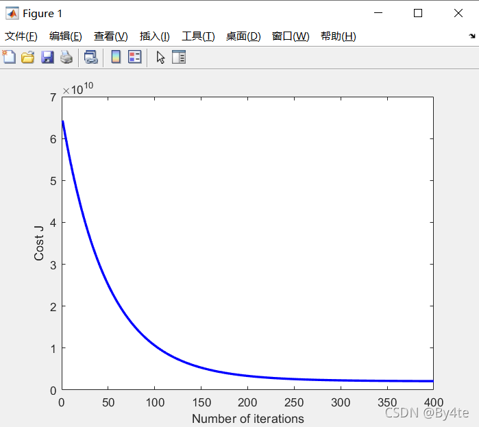
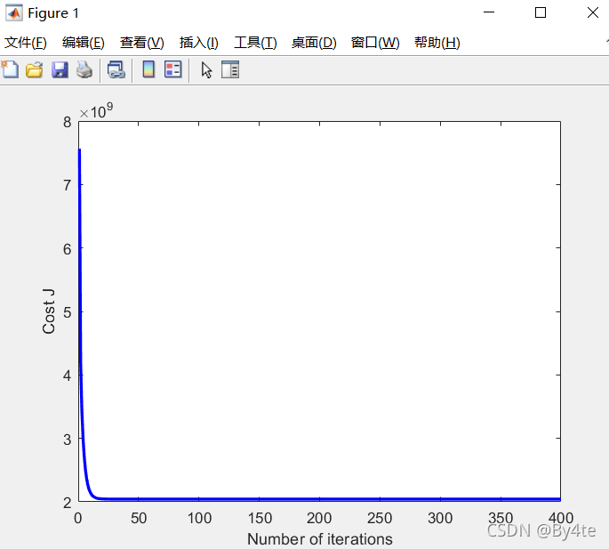
梯度下降代码如下:
fprintf('Running gradient descent ...\n');

alpha = 1.2;                        % 学习率
num_iters = 400;                    % 迭代次数

theta = zeros(3, 1);
[theta, J_history] = gradientDescentMulti(X, y, theta, alpha, num_iters);

figure;
plot(1:numel(J_history), J_history, '-b', 'LineWidth', 2);
xlabel('Number of iterations');
ylabel('Cost J');                                            % 代价函数图像

fprintf('Theta computed from gradient descent: \n');
fprintf(' %f \n', theta);
fprintf('\n');

predict_x=[1650,3];                                        % 预测房价
predict_x=(predict_x-mu)./sigma;
price=[1,predict_x]*theta;

fprintf(['Predicted price of a 1650 sq-ft, 3 br house ' ...
         '(using gradient descent):\n $%f\n'], price);

fprintf('Program paused. Press enter to continue.\n');
pause;
3.3 正规方程
线性回归封闭形式解如下:

使用该公式时无需进行特征缩放,将直接得到精确解
代码如下:
function [theta] = normalEqn(X, y)

theta = zeros(size(X, 2), 1);

theta=pinv(X'*X)*X'*y


end
通过正规方程找到的θ与梯度下降找到的θ进行预测的结果相同
ex1_multi.m代码如下:
clear ; close all; clc
fprintf('Loading data ...\n');
data = load('ex1data2.txt');
X = data(:, 1:2);
y = data(:, 3);
m = length(y);
% Print out some data points
fprintf('First 10 examples from the dataset: \n');
fprintf(' x = [%.0f %.0f], y = %.0f \n', [X(1:10,:) y(1:10,:)]');
fprintf('Program paused. Press enter to continue.\n');
pause;
fprintf('Normalizing Features ...\n');
[X mu sigma] = featureNormalize(X);
X = [ones(m, 1) X];
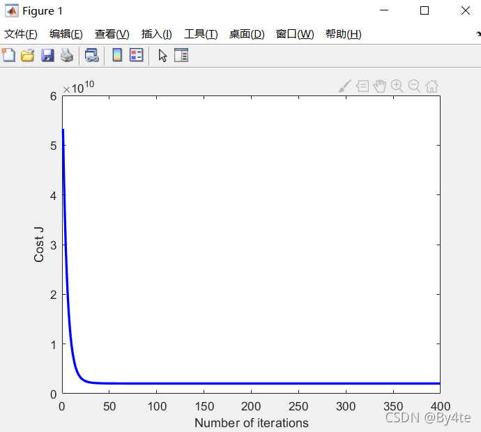
fprintf('Running gradient descent ...\n');
alpha = 1.2;
num_iters = 400;
theta = zeros(3, 1);
[theta, J_history] = gradientDescentMulti(X, y, theta, alpha, num_iters);
figure;
plot(1:numel(J_history), J_history, '-b', 'LineWidth', 2);
xlabel('Number of iterations');
ylabel('Cost J');
fprintf('Theta computed from gradient descent: \n');
fprintf(' %f \n', theta);
fprintf('\n');
predict_x=[1650,3];
predict_x=(predict_x-mu)./sigma;
price=[1,predict_x]*theta;
fprintf(['Predicted price of a 1650 sq-ft, 3 br house ' ...
'(using gradient descent):\n $%f\n'], price);
fprintf('Program paused. Press enter to continue.\n');
pause;
fprintf('Solving with normal equations...\n');
data = csvread('ex1data2.txt');
X = data(:, 1:2);
y = data(:, 3);
m = length(y);
X = [ones(m, 1) X];
theta = normalEqn(X, y);
fprintf('Theta computed from the normal equations: \n');
fprintf(' %f \n', theta);
fprintf('\n');
price=[1,1650,3]*theta;
fprintf(['Predicted price of a 1650 sq-ft, 3 br house ' ...
'(using normal equations):\n $%f\n'], price);
结果如下:
Loading data ...
First 10 examples from the dataset:
x = [2104 3], y = 399900
x = [1600 3], y = 329900
x = [2400 3], y = 369000
x = [1416 2], y = 232000
x = [3000 4], y = 539900
x = [1985 4], y = 299900
x = [1534 3], y = 314900
x = [1427 3], y = 198999
x = [1380 3], y = 212000
x = [1494 3], y = 242500
Program paused. Press enter to continue.
Normalizing Features ...
Running gradient descent ...
Theta computed from gradient descent:
340412.659574
110631.050279
-6649.474271Predicted price of a 1650 sq-ft, 3 br house (using gradient descent):
$293081.464335
Program paused. Press enter to continue.
Solving with normal equations...
Theta computed from the normal equations:
89597.909544
139.210674
-8738.019113Predicted price of a 1650 sq-ft, 3 br house (using normal equations):
$293081.464335


 3330
3330


 被折叠的 条评论
为什么被折叠?
被折叠的 条评论
为什么被折叠?
 到【灌水乐园】发言


