双指数平滑法一例

缘起

某日，一好友给我发了国外运筹学的一个小作业，共三题，问我是否有想法，看了一眼，看到了第一题是之前接触过的时间序列分析，便只做了这一道题，我也是在此过程中第一次接触到了双指数平滑法。(文章未写完，后续会更新)

双指数平滑法

我的参考资料来自 https://support.minitab.com/zh-cn/minitab/18/help-and-how-to/modeling-statistics/time-series/how-to/double-exponential-smoothing/methods-and-formulas/methods-and-formulas/
双指数平滑法是指数平滑法中的一种

题目

Question 1. [40 marks] A time series dataset is provided in the Excel file “data.xlsx”
which contains 156 data points.
(1) Describe the dataset. Consider various aspects, for example the graph, the
“pattern”, the trend, etc.
(2) Treat the data points as they follow a linear trend model. Generate $F_{157}$, $F_{158}$, … , $F_{208}$ by using Double Exponential Smoothing method with $S_0$ = 30, $B_0$ = 10, α = 0.3, β = 0.1 and present the forecasts and real observations in one graph. Round your answers to 3 decimal places. Conceptually do you think this is appropriate for this particular dataset? Why?
(3) Use a different way to produce $F_{157}$, $F_{158}$, … , $F_{208}$ and make a comparison with your result in (2), provide sufficient explanation/reasoning. Again present the forecasts and real observations in one graph. Round your answers to 3 decimal places.

题目解答

（1）To plot the graph, we need to import and preprocess our data first

library(readxl)
library(TSA)
library(forecast)
data <- read_excel("CW Forcasting_Data_update.xlsx", col_names = FALSE)
data = ts(data[2])
colnames(data)[1] = 'measure'
View(data)
plot(data, xlab = 'time', ylab = 'measure', cex = 0.6, type = 'o')

get the graph:

From the graph, we can get

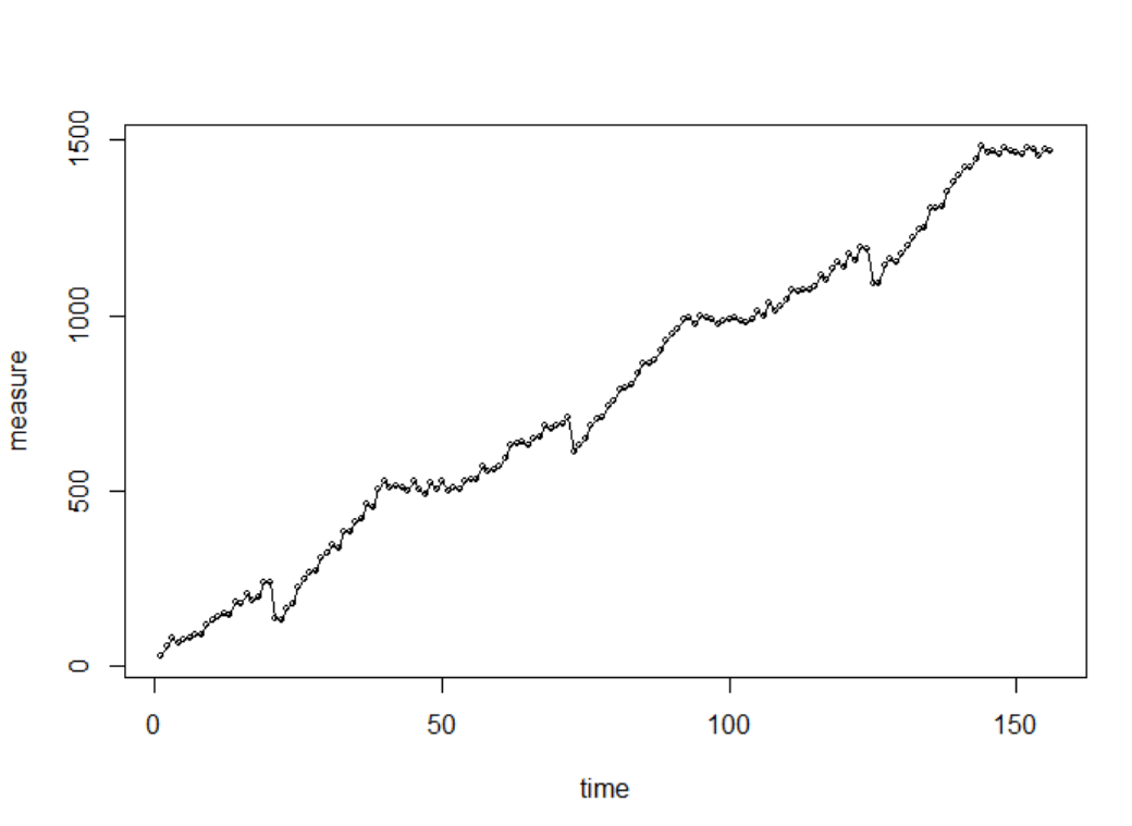
• the graph has a increasing trend
• the graph is not simply linearly increaing, the preiodity can not be ignored
• maybe a seasonal model can be fit

(2) Use function HoltWinters() in R,

data_fit = HoltWinters(data, alpha = 0.3, beta = 0.1, l.start = 30, b.start = 10, gamma = F)
plot(data_fit, xlab = 'time', ylab = 'measure', cex = 0.6, type = 'o')
# Version 8.1 has not reported funvtion “forecast.HoltWinters”,use forecast() instead
data_pre <- forecast(data_fit, h=52)
plot(data_pre)
data_pre

get the graphs:

> data_pre
    Point Forecast    Lo 80    Hi 80    Lo 95    Hi 95
157       1494.277 1451.992 1536.562 1429.607 1558.947
158       1499.746 1455.218 1544.274 1431.646 1567.846
159       1505.214 1458.156 1552.273 1433.245 1577.184
(后面的数据篇幅长，不进行展示)

The column “Forecast” is the result we want.
I think the result is not so good, there’re two main reasons:

• the greatest default is that the preditions has not shown its preiodity, it just show its increaing trend
• the confidence interval and the predition interval are not satisfying

（3）we use function auto.Arima() in R to seek for a better result

data_fit2 <- auto.arima(data)
data_fit2
data_pre2 <- forecast(data_fit2, h=52)
data_pre2

information of the model

> data_fit2
Series: data 
ARIMA(0,1,0) with drift 

Coefficients:
       drift
      9.2839
s.e.  1.8794

sigma^2 estimated as 551:  log likelihood=-708.6
AIC=1421.2   AICc=1421.28   BIC=1427.29

To be honest, the values of AIC and BIC are also not good, let alone it, we next see the prediction, whatever we choose our model, the final goal must a good prediction.

par(mfrow = c(2,1))
plot(data_fit2, xlab = 'time', ylab = 'measure', cex = 0.6, type = 'o')
plot(data_pre2)

The left graph is similar to (2), but the right one get a higher score!
Compare the prediction of $F_{157}$, $F_{158}$, … , $F_{208}$:

The confindence interval and prediction interval significantly reduced .
And the predictions are:

> data_pre2
    Point Forecast    Lo 80    Hi 80    Lo 95    Hi 95
157       1477.284 1447.200 1507.368 1431.275 1523.293
158       1486.568 1444.023 1529.113 1421.501 1551.634
159       1495.852 1443.745 1547.958 1416.162 1575.542
(后面的数据篇幅长，不进行展示)

The column “Forecast” is the result we want.

数据

1	29
2	59
3	79
4	69
5	77
6	81
7	88
8	90
9	119
10	131
11	139
12	149
13	147
14	184
15	180
16	205
17	187
18	198
19	238
20	239
21	138
22	131
23	163
24	178
25	223
26	250
27	266
28	273
29	308
30	321
31	346
32	336
33	384
34	383
35	410
36	419
37	463
38	453
39	507
40	528
41	511
42	515
43	508
44	500
45	526
46	505
47	493
48	524
49	505
50	526
51	501
52	510
53	507
54	529
55	532
56	531
57	568
58	558
59	563
60	570
61	593
62	629
63	636
64	638
65	629
66	649
67	655
68	685
69	677
70	688
71	689
72	710
73	611
74	629
75	651
76	685
77	703
78	710
79	744
80	755
81	787
82	793
83	803
84	838
85	864
86	863
87	874
88	902
89	927
90	946
91	960
92	990
93	993
94	974
95	997
96	995
97	991
98	974
99	984
100	989
101	995
102	987
103	982
104	991
105	1014
106	1000
107	1038
108	1014
109	1026
110	1045
111	1074
112	1067
113	1075
114	1073
115	1082
116	1117
117	1100
118	1133
119	1153
120	1141
121	1178
122	1159
123	1195
124	1189
125	1093
126	1094
127	1142
128	1160
129	1155
130	1175
131	1201
132	1224
133	1247
134	1251
135	1306
136	1308
137	1310
138	1351
139	1381
140	1401
141	1423
142	1421
143	1447
144	1485
145	1467
146	1472
147	1462
148	1480
149	1468
150	1466
151	1460
152	1480
153	1473
154	1457
155	1475
156	1468